Pooling in Graph Neural Networks (1/3)

This post is divided in three parts:

Part 1

Graph Neural Networks (GNNs) have emerged as powerful tools for modeling and analyzing graph-structured data, finding applications across diverse fields like social network analysis, bioinformatics, and recommender systems. Despite their success, scaling GNNs to handle larger and more complex graphs remains a significant challenge. Graph pooling plays a crucial role in enhancing their performance and making them more applicable to a larger class of datasets and applications.

In this post I will give a gentle introduction to pooling in GNNs and an overview of the main families of existing graph pooling approaches. Then, I will present some possible ways to evaluate how good a pooling method is. As the focus in on a tutorial exposition, I will cover only a representative subset of all methods that exist in the literature. I also have tried to keep the notation and the nomenclature as uniform as possible, even if there is quite some variance in the literature.

In this part, I will give a brief introduction to GNNs, graph pooling, and to a general framework for expressing a generic graph pooling operator.

Let’s start!

❶ An introduction to pooling in GNNs

Before talking about pooling in GNNs let’s look at how pooling works in more traditional deep learning architectures, such as a Convolutional Neural Network (CNN).

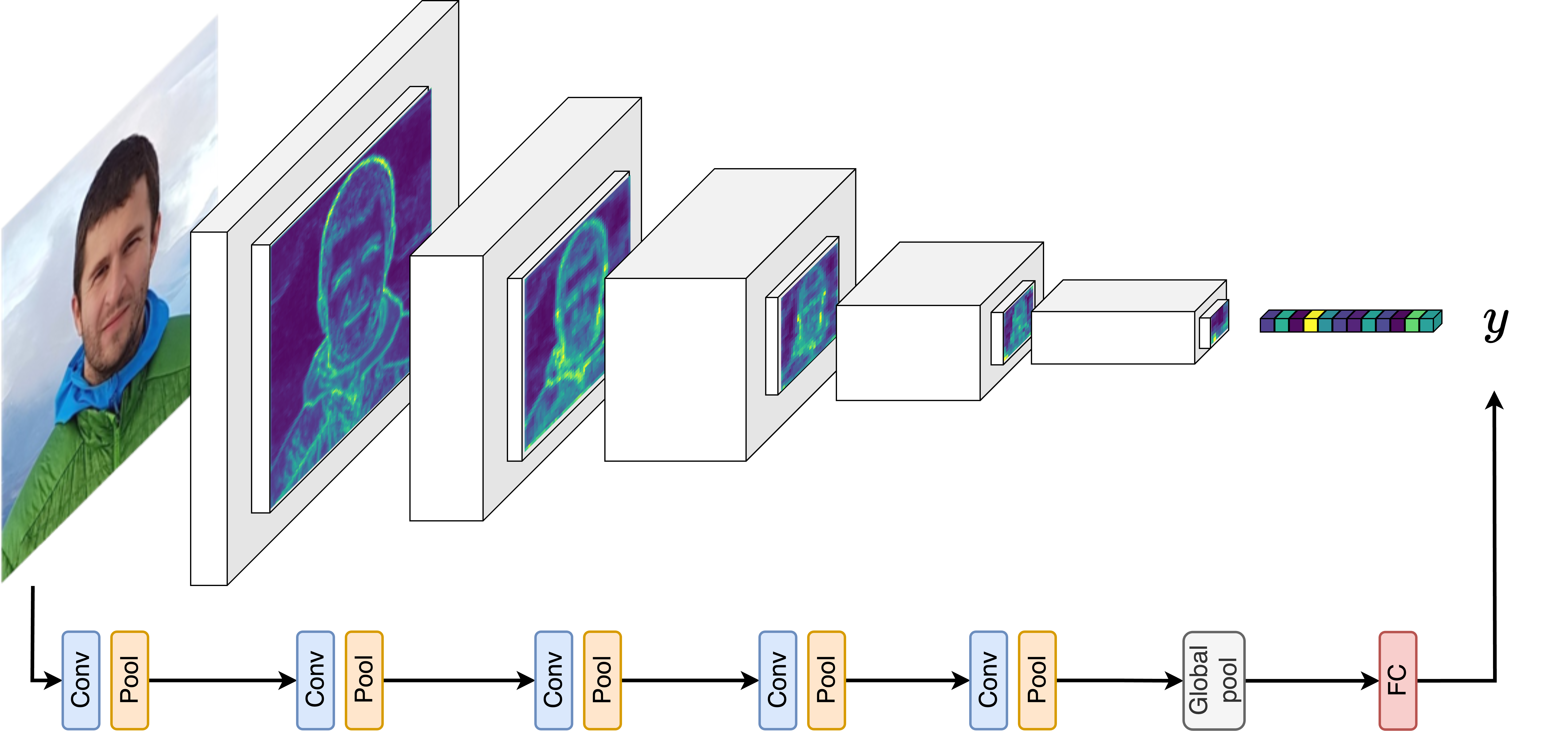
VGG16 architecture — Architecture of VGG16, a traditional CNN for image classification. Blocks of convolutional layers are interleaved with pooling layers that gradually reduce the spatial dimensions of the feature maps.

A standard CNN alternates blocks of convolutional layers, which capture more and more complex features within the image, with pooling layers. The latter gradually reduce the spatial dimensions until the whole image can be squeezed into a (long) vector. Such a vector is then digested by a classifier that produces in output the (hopefully) desired class of the input image.

So, how does pooling work in this case? It simply produces a summary of adjacent pixels in the image. Depending on the function used to produce the summary one obtains different effects. Let’s consider Max and Average pooling, which are the most common ones.

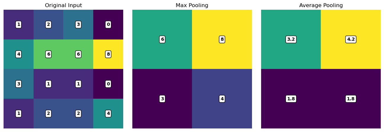
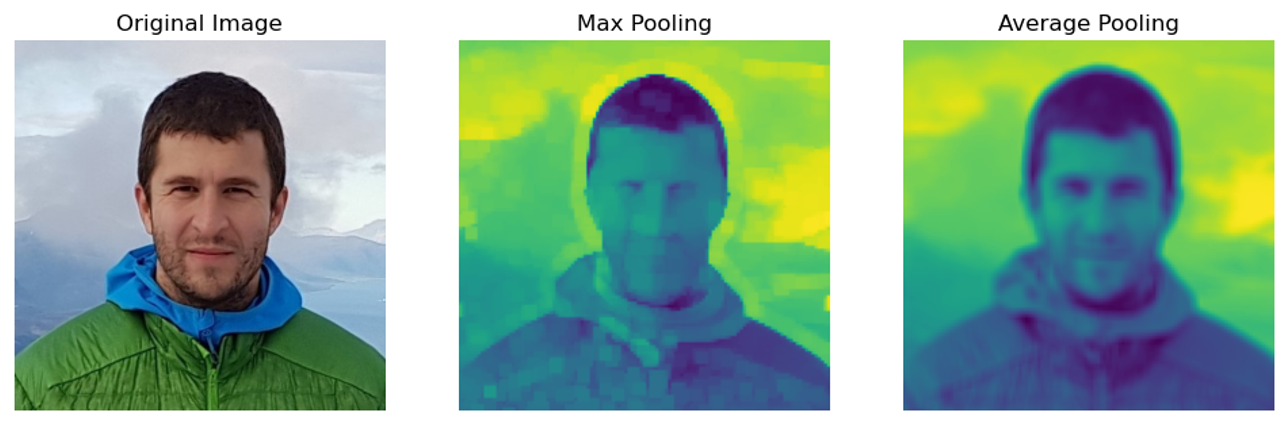
Pooling kernels illustrated on colored squares — Effect of applying **Max** and **Average** pooling on the same image.

Result of Max and Average pooling on a face image — Effect of applying **Max** and **Average** pooling on the same image.

With Average pooling the neighboring pixels are averaged and one ends up with a blurry pooled image. If, instead, one takes the maximum among the patch of neighboring pixels, the obtained effect is that edges are enhanced and that the pooled image looks more sharp and flat. The final effect depends also on other factors, such as the kernel width (i.e.,how many pixels are pooled together) and the stride (i.e., how far apart on the image are the patches of pixels that are pooled). But let’s leave these technicalities aside for now.

Let’s see how these concepts extend to the graph domain by introducing the idea of graph convolutions and message passing.

Graph Neural Networks

The backbone of a GNN is the message passing (MP) layer. For each node, the MP layer learns a new representation using a function $f$, which usually has some trainable parameters.

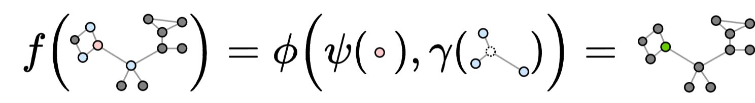
Template formula for a generic MP layer.

In the most general case, $f$ is given by the composition of:

a function $\psi$ that processes the features of the central node 🔴,
a function $\gamma$ that processes the features of the neighboring nodes 🔵,
a function $\phi$ that combines the outputs of $\psi$ and $\gamma$ and produces the output feature 🟢.

Think at this definition of MP layer as a sort of template or abstract class from which a specific MP layer inherits. This is what is actually done in code by popular libraries for GNNs such as PyTorch Geometric.

Flat GNNs

The basic GNN architecture is obtained by stacking multiple MP layers, one after the other.

A “flat” GNN architecture, given by stacking MP layers one after the other.

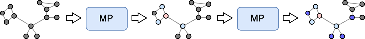
Every time we add an MP layer, we combine the features of a node with those of nodes that are further away on the graph. This is a bit like stacking convolutional layers on top of each other in a CNN, which has the effect of increasing the total receptive field, i.e., the size of the region of the image considered by the CNN to compute the new features. We refer to this type of GNN architectures as flat as opposed to the ones with pooling layers, which we’ll see in a second, that form a hierarchy of intermediate graphs that get smaller and smaller. Flat GNNs do not modify the size of the input graph, which remains always the same. Even if each MP layer can learn more and more complex node representations, the total “receptive field” of the GNN grows rather slowly, similarly to a CNN without pooling layers.

A hierarchical GNN architecture, with pooling layers between the MP layers.

To reach the desired receptive field one should stack many MP layers, but this comes with a few issues. First, we risk to increase too much the model capacity, i.e., the number of trainable parameters, which can lead to overfitting. In addition, repeatedly applying MP can create a problem called oversmoothing, were all node features end up being too similar. Finally, since the nodes of a graph are not independent, it is not trivial to break down a graph into mini-batches for training a GNN like other deep learning architectures. Therefore, one often has to handle the whole graph at once. If the graph is large, applying several MP layers can be computationally demanding and it would be beneficial to gradually reduce its size.

Note
A “flat” GNN that stacks many MP layers can lead to overfitting and oversmoothing and be computationally demanding.

Hierarchical GNNs

Let’s now focus on a GNN that alternates MP layers with pooling layers. We refer to this type of architecture as hierarchical. Like in CNNs, pooling layers reduce the spatial dimension by generating an intermediate structure, which for a GNN is a smaller graph rather than a smaller grid. This allows to expand more quickly the receptive field of the GNN and to extract more easily global properties of the graph such as its class.

What kind of downstream tasks can be solved with hierarchical GNNs?

A lot of them! Let’s see the principal ones.

Graph-level tasks

Graph regression and classification are the most common graph-level tasks. These tasks closely resembles image classification, also in terms of the structure of the deep learning architecture: an alternation of MP/convolutions and pooling layers.

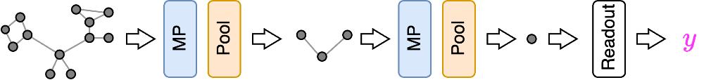
A graph-level task consists in predicting an output $y$, which can be either a real number (e.g., a property of the molecule represented by the graph) or a categorical value (e.g., the class of the graph). A classic example consists in determining if a molecular graph is mutagenic ($y=1$) or not ($y=0$). For this task, the pooling layers help to gradually distill the global property $y$ from the graph.

Node-level tasks

These tasks include node classification and node regression, i.e., predicting for each node $n$ a label $y_n$, which could be the class (node classification) or a numerical property (node regression). A classic example is that of citation networks, where nodes represent articles and their corpus, graph edges represent citations, and the task is to determine the class of some unlabelled nodes/articles.

Node-level tasks are usually performed using flat GNNs architectures. After all, the classification has to be done is the same node space of the input data. If we reduce the graph size with pooling how do we go back? To do that, architectures such as the Graph U-Nets¹ adopt a hierarchical GNN that learns a latent low-dimensional graph representation with graph pooling. Afterwards, the latent representation is mapped back to the original node space through an unpooling (also called lifting) operation, which is complementary to the pooling operation.

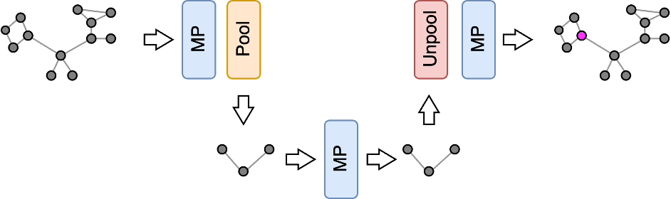
These kind of architectures are similar to the U-Nets used in computer vision to perform image segmentation² or image generation with diffusion models³. Indeed, the latter are pixel-level tasks where the outputs (a segmentation mask or a denoised image) have the same spatial dimension of the inputs.

Even more similar to the Graph U-Nets are the graph filter banks⁴. A filter bank is a collection of filters that decompose a graph signal into different frequency components, typically by applying different graph-based operations such as graph Fourier transform⁵ and graph coarsening⁶. Note that graph coarsening is often used as an acronym for graph pooling especially in the graph signal processing literature.

Note
Graph coarsening is the term used in the signal processing community for graph pooling.

Community-level tasks

This task consists in detecting communities by clustering together nodes that have similar properties or that are strongly connected to each other. As we will see later, some (but not all!) pooling methods can be used for this purpose.

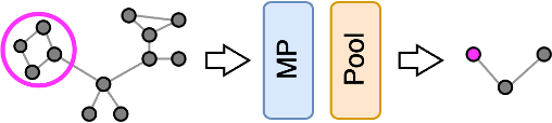
The GNN architecture used to perform this task is very simple: it just consists of one or more MP layers followed by a pooling layer.

GNN architecture used to detect communities.

❷ A general framework for graph pooling

Now that we have seen how to use a pooling operator within GNN architectures that solve different types of task, it is time to address the elephant in the room:

How to compute a pooled graph?

This is a difficult question to answer because there are many different approaches for doing it and none of them is necessarily and always better than the others. It depends on what we want to achieve, what kind of graphs we are dealing with, how large they are, how much computing resources we have, and so on.

The problem of graph pooling, or graph coarsening, is an active area of research. And that’s not all. The problem of how to reduce a graph took different names and perspectives in many different disciplines, including machine learning, signal processing, discrete mathematics, optimization, linear algebra, and even statistics.

To handle this variety of approaches and to provide a formal definition of graph pooling, a few years ago we proposed a general framework called Select-Reduce-Connect (SRC)⁷. SRC is a sort of template that allows us to express any graph pooling operators. This framework is now commonly adopted in the graph pooling community and it’s implemented in deep learning libraries such as PyTorch Geometric and Spektral. Let’s see what SRC is about!

In SRC, a generic graph pooling operator is given by the composition of three functions: Select ($\texttt{SEL}$), Reduce ($\texttt{RED}$), and Connect ($\texttt{CON}$). Let’s say that our original graph has $N$ nodes and the node features of these nodes are stored in a set $\mathcal{X}$. Similarly, the graph has $E$ edges and the edge features are in a set $\mathcal{E}$. In the example below, the original graph has $N=5$ nodes and $E=5$ edges. Let’s also say that the pooled graph has $K$ supernodes with features $\mathcal{X}’$, while the edge features are stored in a set $\mathcal{E}’$. In the example, the pooled graph has 3 supernodes and 2 edges.

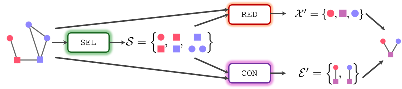
The SRC framework can be used to describe a generic graph pooling operator.

Select

The $\texttt{SEL}$ function is responsible to decide how many supernodes the pooled graph will have and which nodes of the original graph will end up in which supernode. For examples, the nodes {🔴, 🟥} will end in the first supernode, the nodes { 🟥 , 🟦} will be assigned to the second supernode, and the nodes {🟦, 🔵, 🔵} to the third. This can be summarized by the output of $\texttt{SEL}$ as $\mathcal{S}$ = {{🔴, 🟥}, { 🟥 , 🟦}, {🟦, 🔵, 🔵}}. Basically, $\texttt{SEL}$ determines which nodes are selected and how they are grouped together. Note that $\texttt{SEL}$ can also selects only a subset of the whole nodes and discard the others. For example, the output of $\texttt{SEL}$ could be $\mathcal{S}$ = {{🔴}, {🟦, 🔵}}, meaning the the pooled graph has $K=2$ supernodes. The $\texttt{SEL}$ function function is arguably the most important part of a pooling method. In fact, the specific implementation of the $\texttt{SEL}$ function is what mostly sets the different pooling methods apart.

Reduce

The $\texttt{RED}$ operations is the one responsible for computing the node features $\mathcal{X}’$ of the pooled graph. Each pooling method can implement the $\texttt{RED}$ function differently, but in general the result depends on: the node features $\mathcal{X}$, the topology of the original graph, and on the result $\mathcal{S}$ of the $\texttt{SEL}$ function. For example, let’s say that $\texttt{RED}$ computes the features $\mathcal{X}’$ by taking the sum, the max, or the average of the features of the nodes that are assigned by $\texttt{SEL}$ to the same supernode. We would get something like {🔴, 🟥} → 🔴, { 🟥 , 🟦} → 🟪, {🟦, 🔵, 🔵} → 🔵, i.e., $\mathcal{X}’$ = {🔴, 🟪, 🔵}.

Connect

The $\texttt{CON}$ function is basically the same as $\texttt{RED}$, but it deals with the edges and the edge features of the pooled graph. In particular, $\texttt{CON}$ decides how the nodes of pooled graph are going to be connected and what will end up in the edge features of the pooled graph. As for $\texttt{RED}$, the output of $\texttt{CON}$ depends on the original graph and, clearly, also on $\mathcal{S}$.

As we will see in the following, different families of graph pooling operators share some similarities in how they implement the $\texttt{SEL}$, $\texttt{RED}$, and $\texttt{CON}$ functions.

Note
Almost every graph pooling operator can be expressed through the SRC framework.

❸ Global pooling

In the next part, we will go into the details of the different families of pooling operators. But before doing that, let’s discuss the most simple and basic form of graph pooling: global pooling.

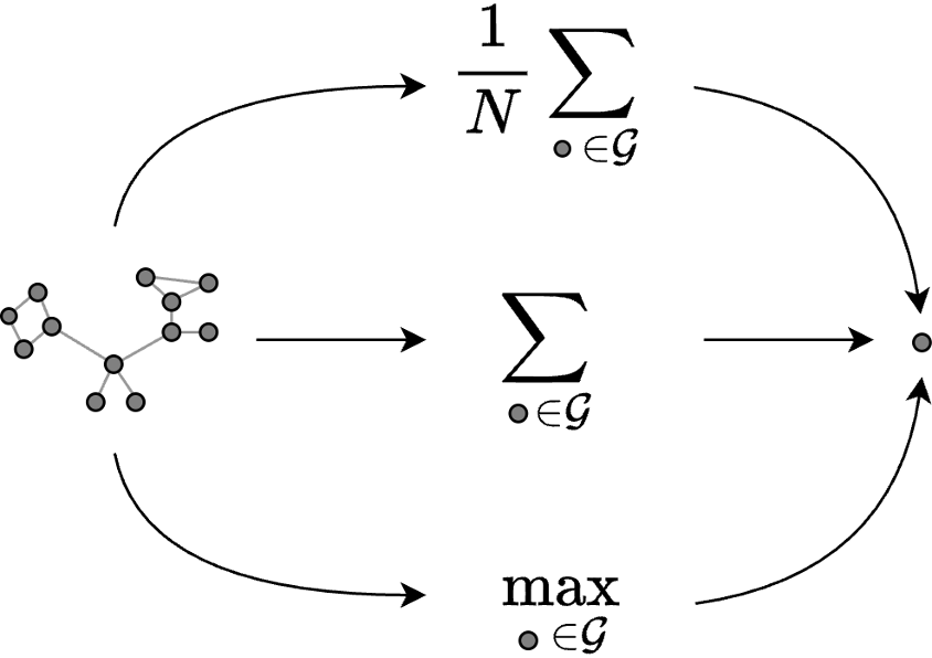
Global pooling operators. They combine all the features of the graph into a single vector, which is the average, the sum, or the maximum of the node features.

Global pooling combines the features from all the nodes in the graph. The output is not a graph but a single node (which, actually, can be seen as a special type of graph) whose features are given by the sum, the maximum, or the average of all the features of the nodes in the graph. Despite being so simple, global pooling is quite useful and popular. For example, is it always used at the end of a GNN for graph-level tasks to combine the features of the remaining nodes. The output is a vectorial representation of the graph that is processed by a classifier to predict the graph class $y$.

We are now ready to delve into the three main classes of hierarchical pooling operators: the soft clustering, the one-over-K, and the score-based pooling methods.

📝 Citation

If you found this useful and want to cite it in your research, you can use the following bibtex.

@misc{bianchi2024intropool
  author = {Filippo Maria Bianchi},
  title = {An introduction to pooling in GNNs},
  year = {2025},
  howpublished = {\url{https://filippomb.github.io/blogs/gnn-pool-1/}}
}