Pooling in Graph Neural Networks (2/3)

This post is divided in three parts:

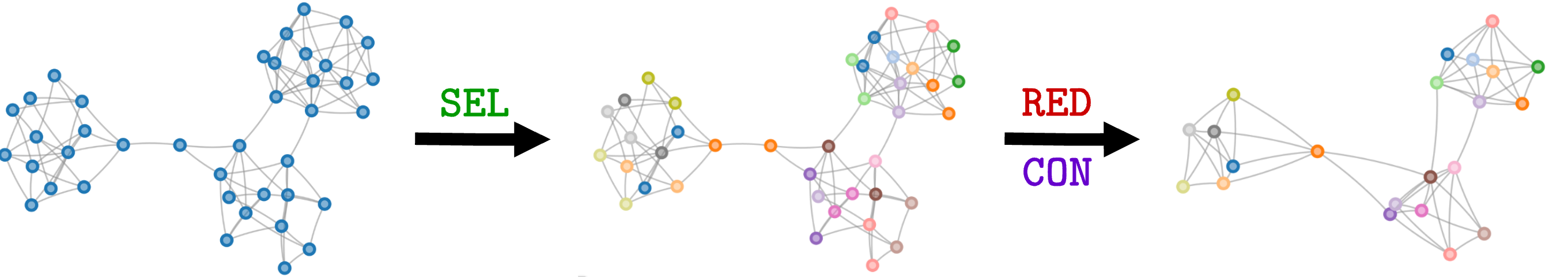
In the first part, I introduced Graph Neural Networks (GNNs) and graph pooling. I also introduced the Select Reduce Connect (SRC) framework, that allows us to define, formally, any graph pooling operator.

In this part, I will discuss the three main families of graph pooling operators.

Part 2

❹ Soft clustering pooling methods

These methods generate a pooled graph by first identifying communities of nodes. The supernodes in the pooled graph are the representatives of such communities. The features of the supernodes are obtained by combining the features of the nodes in the same community. The edges of the supernodes depend on the edges connecting nodes from different communities.

Soft clustering pooling generate a pooled graph from the graph communities.

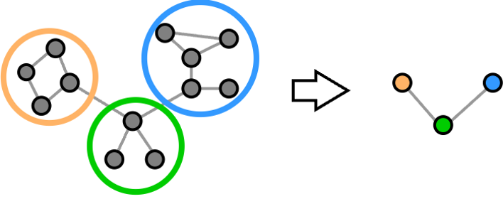
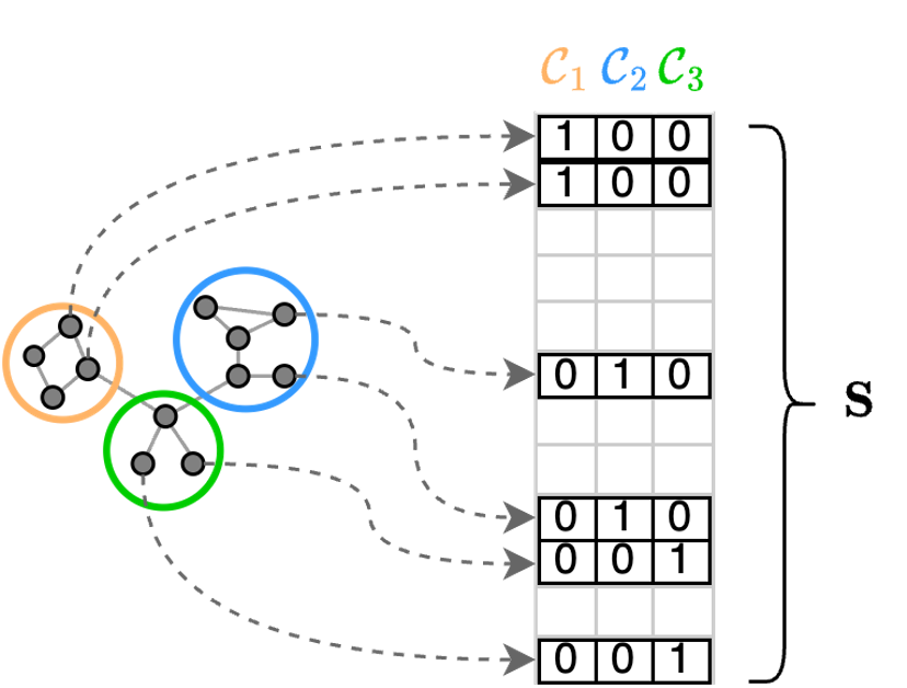
The communities, or clusters, consist of nodes that have similar features or that are strongly connected, i.e., they belong to a section of the graph with high edge density. A partition is what defines how the nodes are assigned to different communities. A partition can be conveniently represented by a cluster-assignment matrix $\mathbf{S}$, which defines to which cluster each node is assigned. The entries of $\mathbf{S}$ can be either 0 or 1. If entry $s_{i,j}=1$ it means that node $i$ is assigned to the community $j$.

A cluster assignment matrix defines the node partition, i.e., how the nodes are assigned to the different communities.

In a GNN, the cluster assignments can be obtained by transforming the node features into the rows of a cluster assignment matrix. In particular, a node feature vector $\mathbf{x}_i \in \mathbb{R}^F$is transformed into the row i-th row $\mathbf{s}_i \in \mathbb{R}^K$of the cluster assignment matrix. This can be done simply by applying a linear transformation followed by a $\texttt{softmax}$

\[\mathbf{s}_i = \texttt{softmax}\left( \mathbf{x}_i \mathbf{W}\right), \; \mathbf{W} \in \mathbb{R}^{F \times K}\]

or by applying a more complex function such as an MLP. The $\texttt{softmax}$ function ensures that the elements in each row $\mathbf{s}_ i$ sums to one. This ensures that the cluster assignments are well-behaved and that all the properties necessary to obtain a proper partition are in place. However, each entry $s_{i,j}$ now assumes a real value in the interval $[0,1]$ rather than being exactly 1 or 0. In other words, we no longer have a crisp cluster assignment, but rather a soft cluster assignment. In this setting, each entry $s_{i,j}$ can be interpreted as the membership of node $i$ to the community $j$. Clearly each node can belong to different clusters with different membership values. For example, if $\mathbf{s}_i = [0.1, 0.6, 0.3]$ node $i$ belongs with membership 0.1 to community 1, with membership 0.6 to community 2, and with membership 0.3 to community 3.

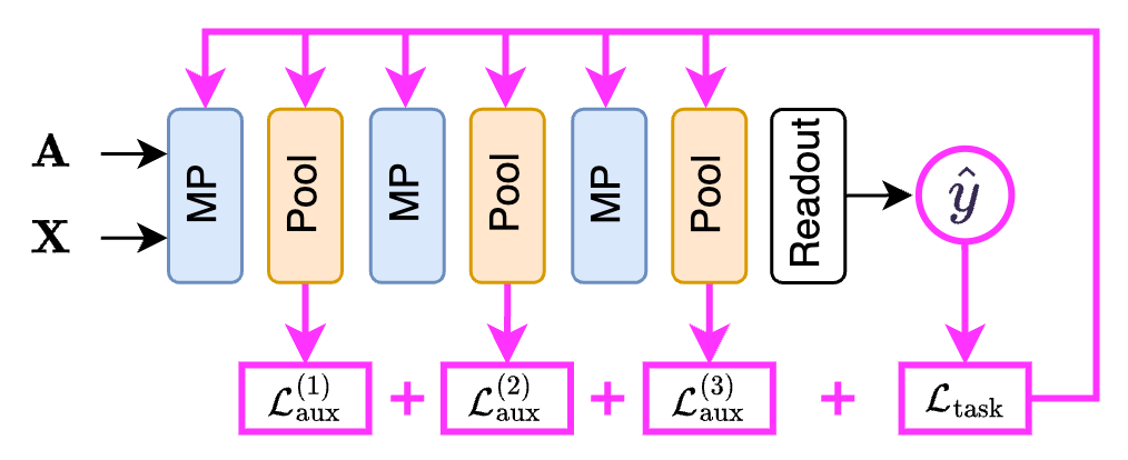
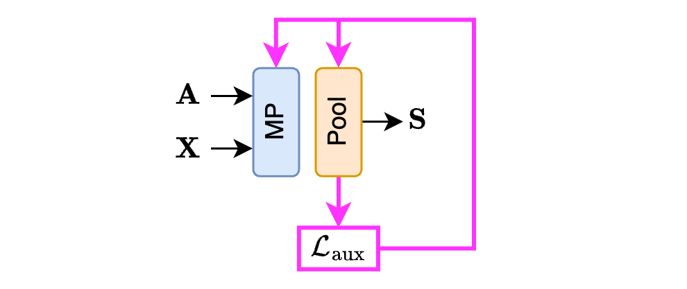
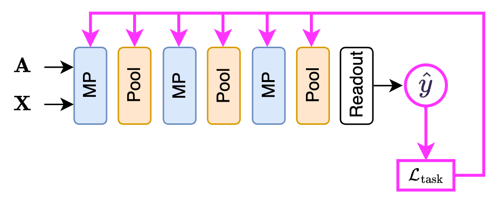
A GNN with a soft clustering pooling layer usually has the following form. First, the usual stack of $L$ MP layers processes the input graph and generates node features $\mathbf{X}^L$. Then, those are processed by a linear (or an MLP) layer to generate the cluster assignments $\mathbf{S}$.

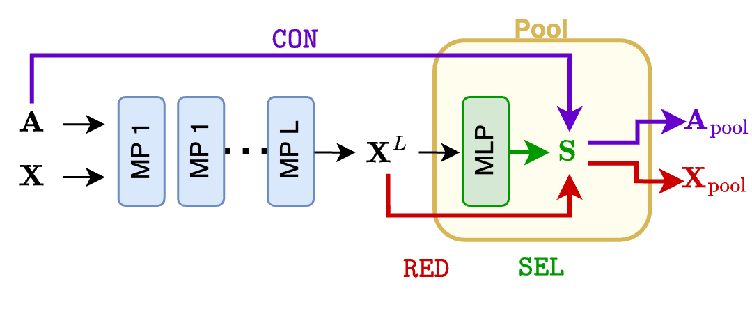
Architecture of a soft clustering pooling layer, highlighting the $\texttt{SEL}$, $\texttt{RED}$ and $\texttt{CON}$ operators.

In soft cluster pooling methods, the $\texttt{SEL}$ function boils down to generating the cluster assignment matrix $\mathbf{S}$. The $\texttt{RED}$ function computes the node features of the pooled graph as

\[\mathbf{X}_\text{pool} = \mathbf{S}^\top\mathbf{X},\]

and the $\texttt{CON}$ function computes the adjacency matrix of the pooled graph as

\[\mathbf{A}_\text{pool} = \mathbf{S}^\top\mathbf{A}\mathbf{S} \;\; \text{or} \;\; \mathbf{A}_\text{pool} = \mathbf{S}^+\mathbf{A}\mathbf{S}.\]

Degenerate solutions

In general, we would like the cluster assignments to be similar if two nodes have similar features and are strongly connected. For this second point, we get help from the block of MPs before the pooling layer that combine the features of a node with its neighbors. Indeed, if there are many paths connecting two nodes $i$ and $j$, the features $\mathbf{x}_i^L$ and $\mathbf{x}_j^L$ generated by the last MP layer will be very similar. This gives us a good starting point to compute the soft cluster assignments because if we pass to the linear layer (or the MLP) two inputs $\mathbf{x}_i^L$ and $\mathbf{x}_j^L$ that are similar, it will produce two outputs $\mathbf{s}_i$ and $\mathbf{s}_j$ that are also similar. This is because the linear layer and the MLP are smooth functions, i.e., they map similar inputs into similar outputs.

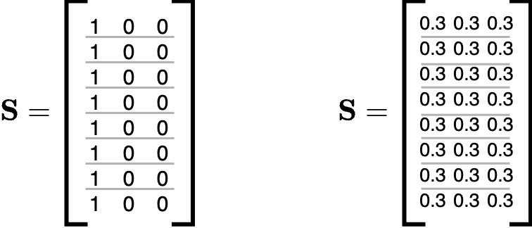
Even if this is a great starting point, unfortunately, it is not enough. The problem is the presence of some degenerate solutions that are commonly encountered when training a GNN with these pooling layers. The first, occurs when all nodes are assigned to the same cluster. The second, is when the nodes are assigned uniformly to all clusters.

Typical degenerate solutions encountered when computing a clustering partition. On the left, a solution that assigns all nodes to the same community. On the right, a solution where the nodes are assigned with the same membership to all communities.

Auxiliary Losses

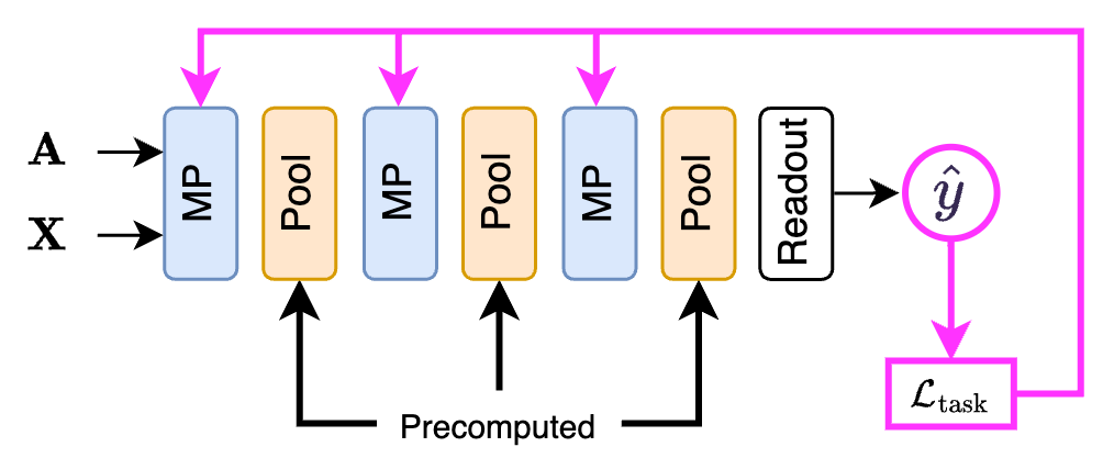
How can these degenerate solutions be avoided? The most effective way is to add an auxiliary loss to each pooling layer that discourages them. The whole GNN is then trained by minimizing the standard loss of the downstream task (a cross-entropy in the case of classification, an MSE in the case of graph regression, etc.) in addition to auxiliary losses associated to the pooling layers:

\[\mathcal{L}_\text{tot} = \mathcal{L}_\text{task} + \sum_i \mathcal{L}_\text{aux}^{(i)}\]

The total loss is used to train the whole GNN, i.e., the parameters of the MP layers and the linear layer/MLP within each pooling layer.

A total loss, given by the combination of the task loss and the auxiliary losses associated with each pooling layer, is used to train the parameters in the MP and pooling layers.

Soft clustering pooling layers are the most versatile among all the pooling layers. In addition to node- and graph-level tasks, they can also be used to perform a community detection task, as we saw in the previous post. In this case, there are no supervised task losses and the GNN is trained only by minimizing the unsupervised auxiliary loss.

A GNN for community detection is trained by optimizing only the unsupervised auxiliary loss.

Summarizing, we have a bunch of auxiliary losses $\mathcal{L}_\text{aux}$ associated with each pooling layer that we use to train the GNN. Let’s now discuss how these auxiliary losses are made.

Each soft clustering pooling method uses different ones. However, despite being different, all the auxiliary losses have something in common. Let us consider four different methods: Diffpool¹, MinCutPool², DMoN³, and TVGNN⁴. Without going into the technicalities of each method, they all use auxiliary losses made of two components:

\[\mathcal{L}_\text{aux} = \mathcal{L}_\text{topo} + \mathcal{L}_\text{quality}\]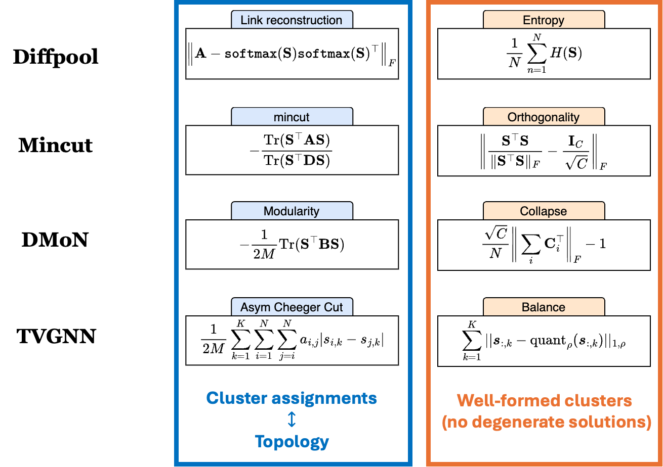

Auxiliary losses of different soft clustering pooling methods. All of them have the same two components. The first, ensures that the cluster assignments are aligned with the graph topology (connected nodes are assigned to the same cluster). The second, monitors the quality of the partition (degenerate solutions are penalized).

The first component, $\mathcal{L}_\text{topo}$, ensures that the cluster assignments are in agreement with the graph topology, i.e., that if two nodes are connected they have the same cluster assignment. As we see from the figure, the loss of each pooling method does something slightly different, but they all try to match the cluster assignments $\mathbf{S}$ with the adjacency matrix $\mathbf{A}$.

The second component, $\mathcal{L}_\text{quality}$, ensures that the clusters are well formed, meaning that the degenerate solutions are avoided. One way of doing this is to ensure that the clusters are balanced (the amount of nodes assigned to each cluster should be similar) and that the cluster assignments resemble a one-hot vector.

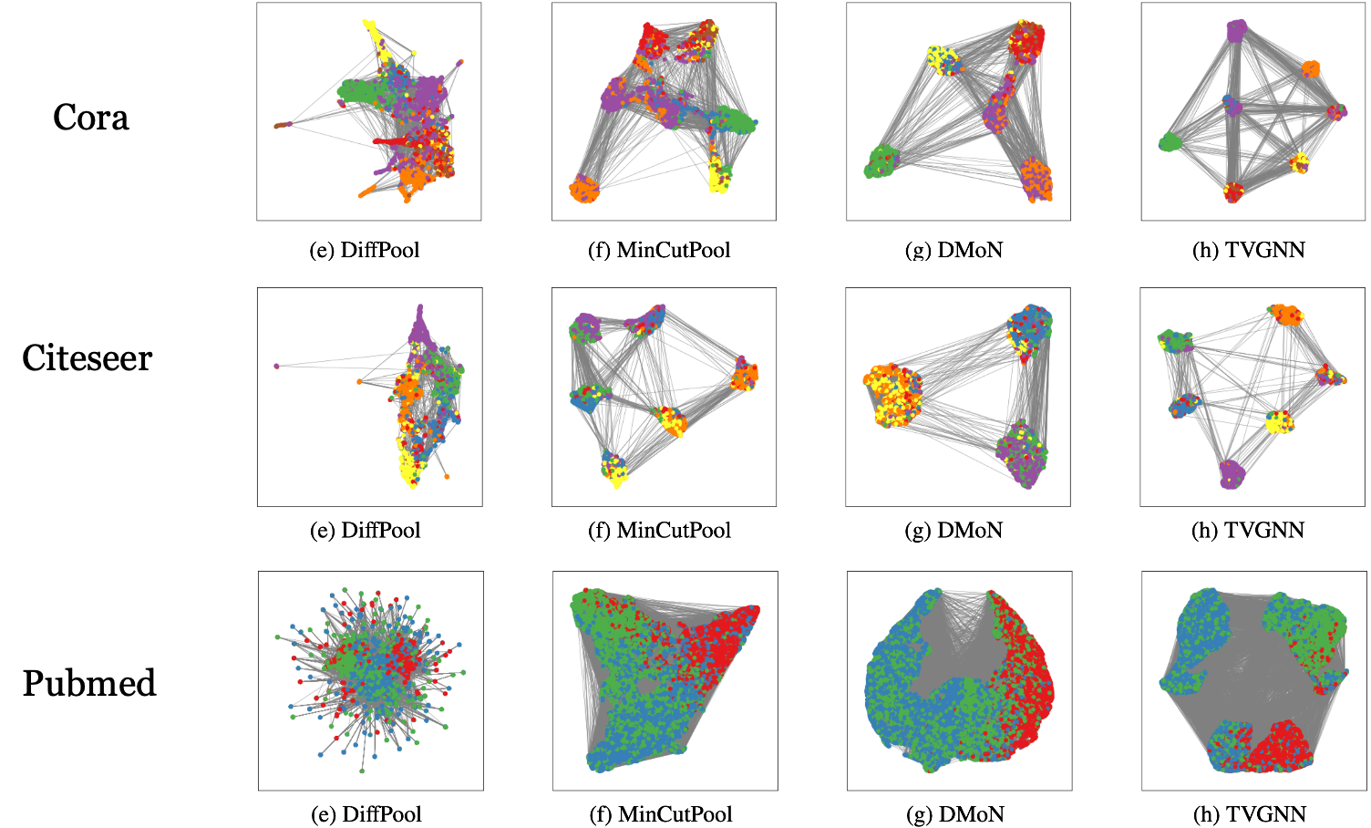
Despite these different losses have the same structure, using one or the other has a profound effect on the final result. To see this, let us consider the community detection task we discussed earlier. As we already mentioned, a soft clustering pooler can be used to solve this task because we can train the GNN in a completely unsupervised way only by minimizing the auxiliary losses, which do not depend on supervised information such as the class label $y$. As we will see later, this is not possible with other types of pooling operators that have no auxiliary losses. Depending on the auxiliary loss, the result of the community detection changes drastically. To see this let’s look at the figure below that shows the communities found on three popular citation networks.

The colors of the nodes in the figure represent the true classes of the nodes. The classes are not seen during the optimization that relies only on the unsupervised auxiliary losses. Ideally, we would like the cluster to be compact and well separated from each other. In addition, we would like that each cluster contains only nodes of the same class, i.e., of the same color.

Pros and Cons

To wrap up, let’s list what are the pros and cons of the soft clustering pooling methods.

Pros.

✅ Thanks to the trainable parameters contained in the linear/MLP layer, soft clustering pooling methods are flexible and can learn to pool the graph in a way that is optimal for the downstream task at hand.

✅ Since each node is assigned to a supernode, the pooled graph preserve a lot of the information of the original graph.

For these reasons, GNNs equipped with soft clustering pooling usually achieve high performance on the downstream tasks.

Cons.

❌ The soft-assignment matrix is dense and can be large, meaning that performing operations such as $\mathbf{S}^\top\mathbf{A}\mathbf{S}$ to compute $\mathbf{A}’$ is expensive. In addition, the pooled adjacency matrix $\mathbf{A}’$ is dense, meaning that the next MP operations operating on the pooled graph cannot exploit sparse operations. For these reasons, soft clustering pooling do not scale well to large graphs.

❌ The number of clusters $K$ must be specified in advance and is fixed. This means that in a graph-level tasks all the pooled graphs end up having the same number of supernodes. This might be a limitation if the dataset contains graphs with very different size. Let say some graphs have 100 nodes, while others have 10, and that we set $K=20$. All pooled graphs will have 20 nodes, meaning that in some extreme cases pooling upscales the size of the graph rather than reducing it. Clearly, this is not desirable. In addition, $K$ is an hyperparameter that, in some cases, might be difficult to choose.

❺ One-over-K pooling methods

The idea of “picking one over K” samples is very straightforward when we think of a sequence or at other regular structures such as a grid. The example below shows how to select 1-every-2 pixels in an image or 1-every-4 samples in a time series.

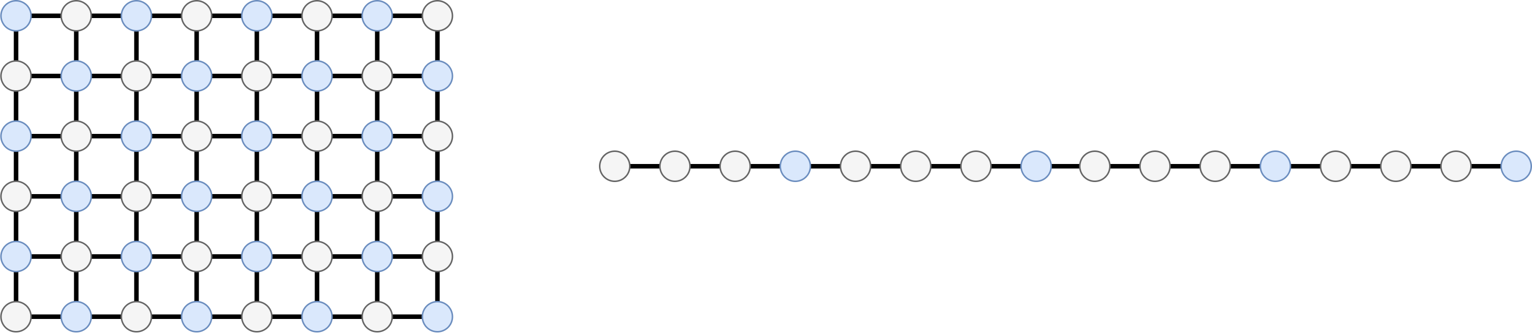
Left: 1-over-2 elements in the grid are selected. Right: 1-over-4 elements of the sequence are selected.

This type of techniques allows to subsample uniformly a data structure, which, in most cases, is a good way to preserve its global structure. However, how can we extend this to graphs? What does it mean to take one node every $K$ nodes? Let’s see it with the following examples.

Graclus

Let’s first consider Graclus⁵, a spectral clustering technique used to progressively aggregate the nodes in a graph. Graclus identifies pairs of nodes that are the most similar according to the graph topology. The two nodes in a pair are merged into a new supernode, which inherits the incoming and outcoming edges of the merged nodes. At the end of this procedure the size of the pooled graph is approximately halved.

According to the SRC framework, the procedure of identifying the pair of nodes to be merged correspond to the $\texttt{SEL}$ function. Note that in Graclus $\texttt{SEL}$ does not look at the node (or edge) features, but accounts only for the graph topology, i.e., the adjacency matrix $\mathbf{A}$.

The $\texttt{SEL}$ function in Graclus finds pairs of nodes to merge only based on the graph connectivity. The features of matched nodes are combined and their edges are coalesced.

The $\texttt{RED}$ function combines the features of the pair of matched nodes. Different options can be used, such as taking the sum, the average of the maximum of the two node features $\mathbf{x}_i$ and $\mathbf{x}_j$. The analogy with the 1-over-2 sampling is best seen if we use the maximum as the aggregation function because we keep a single node in each pair of the matched nodes.

Similarly to $\texttt{RED}$, $\texttt{CON}$ coalesces the edges connected to the matched nodes into new edges. The weight of the new edges can either be the sum, the average or the maximum of the weights of the original edges.

Let’s stress once again that the pooling operations made by Graclus do not depend on the node features but only on the adjacency matrix of the original graph, which is generally not modified while training the GNN. For this reason, it is possible to precompute the coarsened graph in a pre-processing step. Clearly, this greatly speeds up the training. On the other hand, the flexibility of the overall model is limited as it cannot adapt the topology of the pooled graph during training in a way that better optimizes the downstream task. However, this is not always necessarily bad. Fixing the pooling operation in a somewhat reasonable way provides a structural bias to the model. This, could simplify the training in cases where there are a few data available or the learning procedure is particularly difficult. Note that the possibility of precomputing the coarsened graph is common to most one-over-K pooling methods.

Note
The majority of one-over-K pooling methods can precompute the pooled graph in a preprocessing step, which greatly speed up training at the cost of a reduced flexibility.

Node Decimation Pool

The next method in this family is Node Decimation Pool (NDP)⁶. Like Graclus, NDP extends the 1-over-2 concept to graphs. This is done by partitioning the nodes in two sets in a way that there are as much connections as possible between the two sets and as few connections as possible within each set. Note that this is exactly the opposite of what we saw in soft clustering approaches and Graclus! There, the groups contained nodes with many connections.

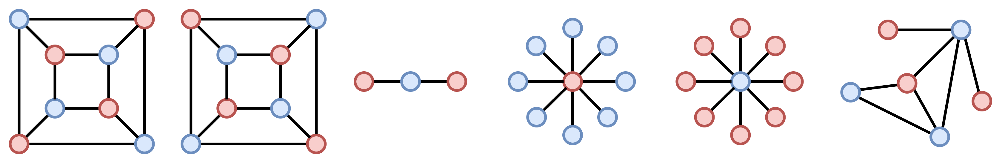
The problem solved by NDP is the same of the MAXCUT, or maximum cut, which tries to find an answer to the following question: “how to color the nodes in a way that as few adjacent nodes as possible have the same color”? If we cut each edge connecting nodes with different colors, we realize that the node coloring problem is the same as to putting in opposite sides of a partition nodes that are connected.

Note that a solution that cuts all the edges exists only in bipartite graphs. An example of a bipartite graph can be found in a recommender system, where the user nodes are connected with the product nodes, but users and products are not connected among them.

Left: an example of a MAXCUT partition, which cuts the edges (in red) that connect nodes belonging to different sides of the partition. Edges connecting nodes of the same color are not cut. The coloring is made in such a way that as many edges as possible are cut. Right: cutting all the edges is possible only in bipartite graphs, such a those in a recommender system.

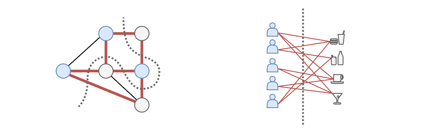
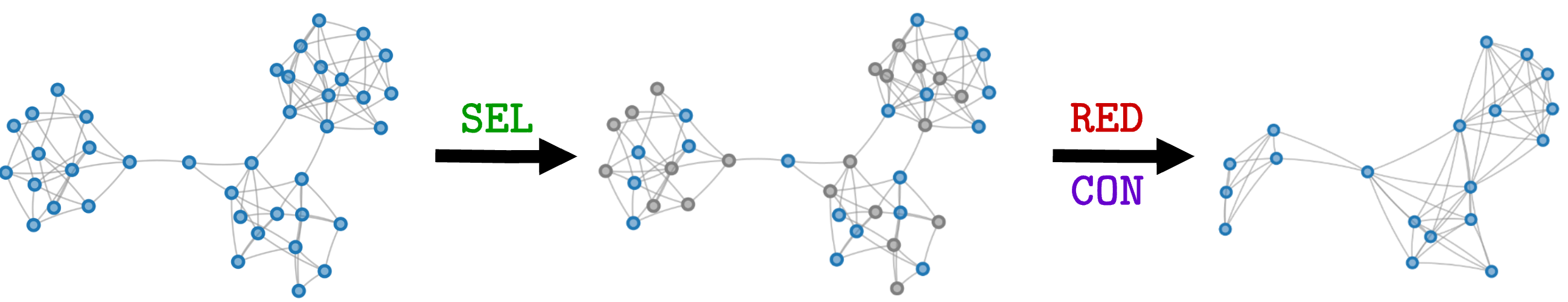
The $\texttt{SEL}$ operation in NDP boils down to doing a coloring that maximizes the number of cut edges. Afterwards, one of the sides of the partition (e.g., the gray nodes) is dropped and the other (blue nodes) is kept. The intuition for why this works is that if two nodes are connected their features will be very similar because they exchanged information during the MP operations. Therefore, keeping both of them is redundant: one type of color can be dropped, while the nodes of the other color becomes the supernodes in the pooled graph.

The $\texttt{SEL}$ operation of NDP partitions the nodes into two sets, such that nodes in the same set are connected as much as possible with nodes from the other set. One side of the partition becomes the nodes of the pooled graph. The $\texttt{RED}$ function simply keeps the features of the selected nodes, while $\texttt{CON}$ uses Kron reduction to connect the pooled nodes.

Finding the MAXCUT (and, by the way, also the mincut) is an optimization problem with combinatorial complexity, meaning that finding the optimal solution is too expensive. For this reason, NDP uses an approximation based on the spectral decomposition of the adjacency matrix that is much more efficient to compute and works well in many cases.

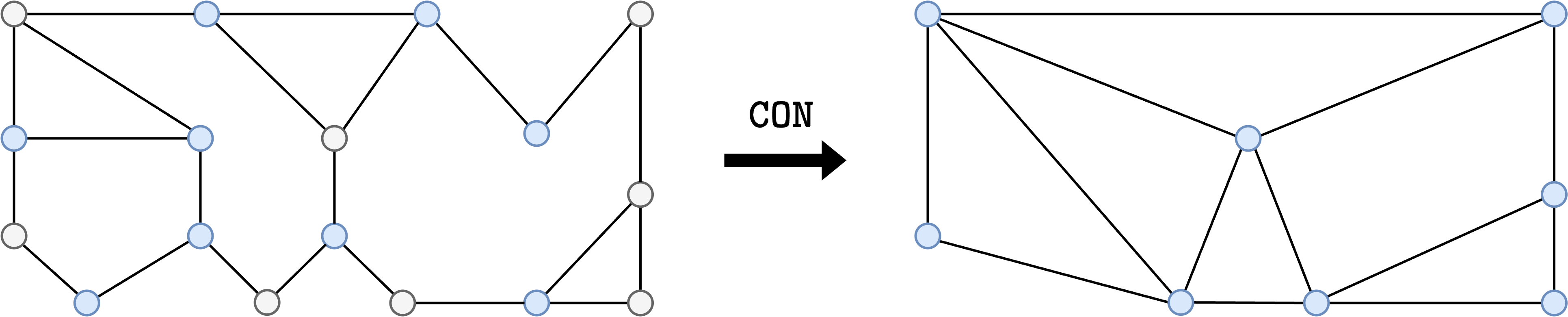
The $\texttt{RED}$ function in NDP does… nothing. The features of the nodes that are kept remain unchanged in the pooled graph. The $\texttt{CON}$ function, instead, is implemented with an algorithm called Kron reduction, which is something used in several fields such as circuit theory⁷. The main idea is that, given a graph with nodes of two different colors (e.g., blue and gray), Kron reduction connects two blue nodes i and j only if in the original graph one can walk from from i to j only visiting gray nodes.

The Kron reduction connects two blue nodes that are originally disconnected only if there are only white nodes between them in the original graph.

Since Kron reduction tends to create very dense graphs, the $\texttt{CON}$ function of NDP applies also a sparsification to remove edges with a small weight in the pooled graph.

Both Graclus and NDP reduce the size of the graph approximately by half, i.e., $N/2$. But what if we want a smaller pooled graph? The only option is to apply pooling in cascade, one after another. This, would make it possible to obtain pooled graphs of size $N/4$, $N/8$, $N/16$, and so on. While applying several times pooling in cascade has a cost, both Graclus and NDP can precompute the pooled graph, so this operation does not really affect the training stage. A drawback, however, is a lack of flexibility in the size of the pooled graph that we get. The next pooling method that we’ll see gives us more flexibility in this respect, as it implements a 1-over-K pooling strategy, differently from the 1-over-2 of Graclus and NDP.

k-Maximal Independent Sets

Here enters k-Maximal Independent Sets (k-MIS) pooling⁸. A maximal independent set is the largest set of vertices in a graph such that no two vertices in that set share an edge. The basic idea of k-MIS pool is that each node in the MIS becomes a supernode of the pooled graph. Note how the problem of finding the MIS is closely related to node coloring and to the MAXCUT objective optimized by NDP⁹. And, just like NDP, k-MIS pool relies on heuristics to find and approximate solution.

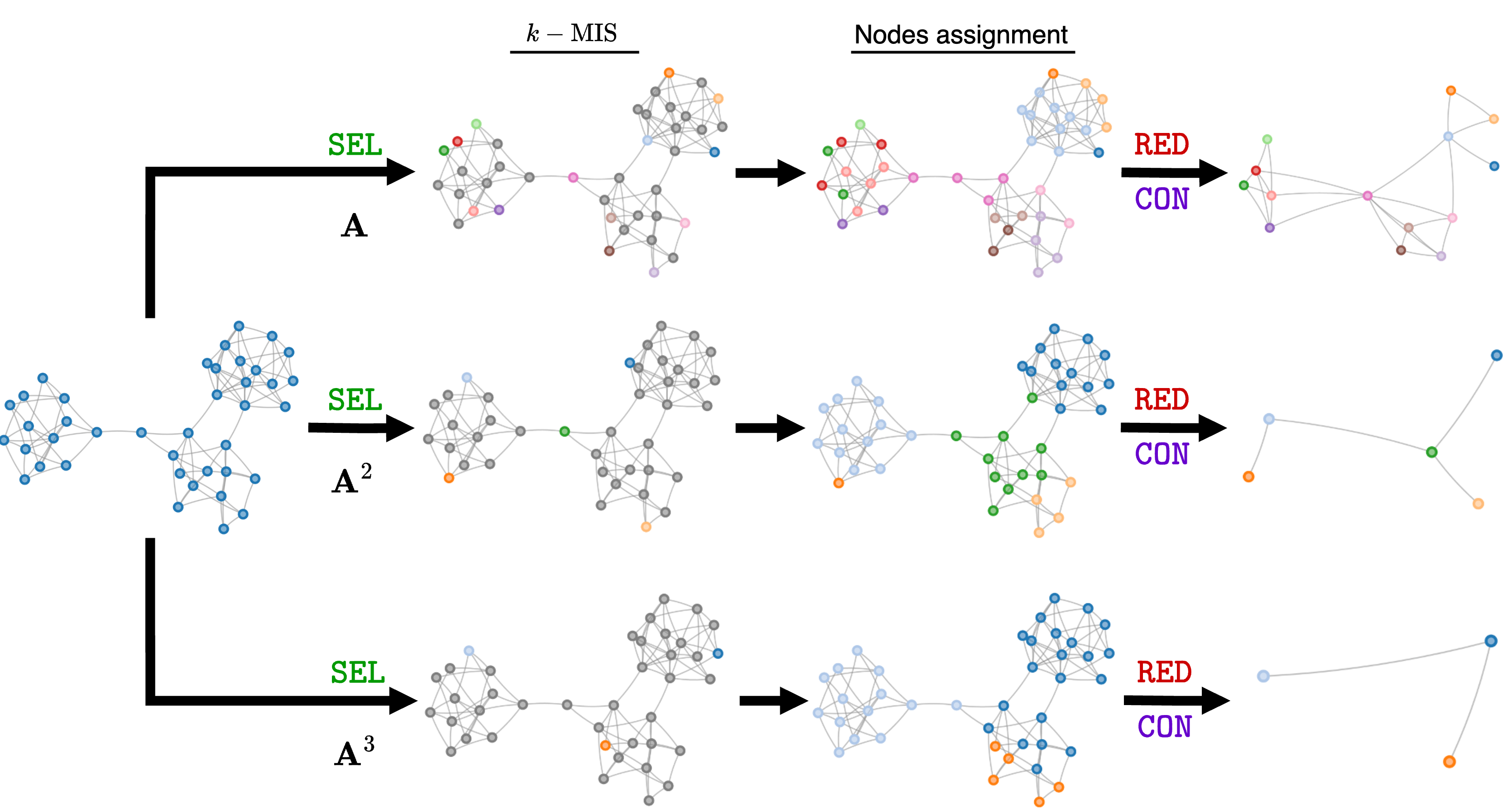
Examples of MIS (nodes in red). By looking at the star graph, we can see how different in size two MIS for the same graph can be.

But what the “k” in k-MIS pool stands for? A set of vertices is said to be k-independent if all vertices it contains have a pairwise distance greater than K. In other words, it takes at least K hops to move to one set to the other in the set. The k-MIS can be conveniently found by computing the MIS on the K-th power of the adjacency matrix $\mathbf{A}^K$. Therefore, k-MIS can produce produce a much more aggressive pooling than Graclus and NDP by using $K=2,3,\dots$

The $\texttt{SEL}$ operation in k-MIS pool consists of two steps:

The nodes of the k-MIS become the supernodes of the pooled graph.
The remaining nodes are assigned to the closest node in the k-MIS.

Similarly to Graclus, the $\texttt{RED}$ function computes the features of the supernodes by taking the sum, average, or max of all the node features assigned to the same supernode. Still like Graclus, $\texttt{CON}$ coalesces the edges of the nodes assigned to the same supernodes to form the new edges.

Pooled graphs obtained with k-MIS pool using values K=1,2 and 3. The higher the K, the more aggressive the pooling.

Since the one-over-K methods do not use auxiliary losses and have no trainable parameters, training a GNN with this kind of pooling layers is pretty straightforward. Like in a flat GNN, we only optimize the weights in the MP layers using the loss from the downstream task. Also, since we have no auxiliary losses, we can use these pooling layers only for graph- and node- level tasks, but not for community detection.

Training of a GNN for graph-level tasks with one-over-*K* pooling layers.

Pros and Cons

To wrap up, let’s summarize the advantages and disadvantages of one-over-K pooling methods.

Pros.

✅ Pooling is precomputed, making training very fast and efficient. This is a good choice when dealing with large graphs or when we do not have enough computing resources.

✅ The lack of trainable parameters introduces a structural bias that simplifies training and allows to reduce the GNN capacity, which is good if we are dealing with small datasets.

Cons.

❌ These methods do lack the flexibility of learning how to pool the graph in a way that is optimal for the downstream task at hand.

❌ They do not account for node features, meaning that they might aggregate in the same way nodes with different or similar features.

❻ Score-based pooling methods

After applying one or more MP layers, the score-based pooling methods project the node features into a score vector $\mathbf{s} \in \mathbb{R}^{N \times 1}.$ Let say that $\mathbf{X}^L \in \mathbb{R}^{N \times F}$ are the node features that we get after applying $L$ MP layers. The score vector is computed by multiplying the node features with a projection operator $\mathbf{p} \in \mathbb{R}^{F \times 1}$ consisting of free, trainable parameters. The nodes associated with the top-K values in $\mathbf{s}$ are selected as the supernodes of the pooled graph. Since the top-K operation that selects the supernodes is not differentiable, to let the gradients flow through the pooling operation the score vector is multiplied element-wise with the features of the pooled nodes.

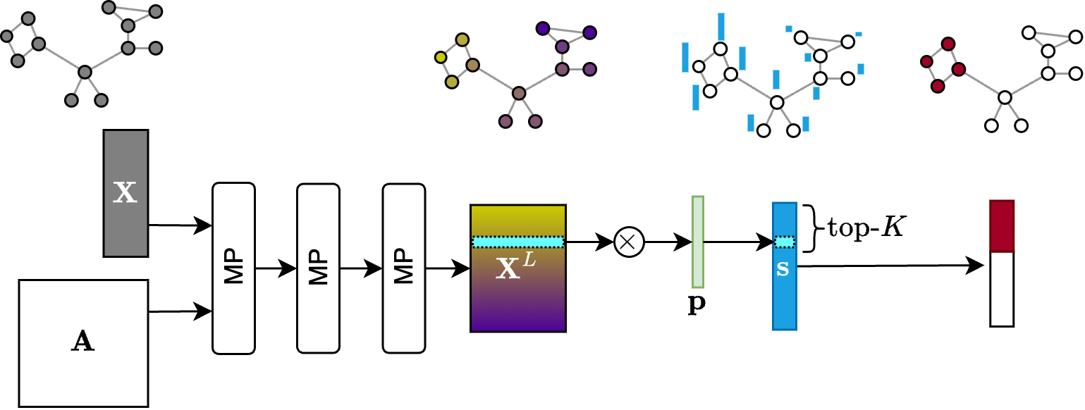
Scheme of the $\texttt{SEL}$ operation in score based methods. The node features produced by a stack of MP layers are mapped by a projection operator into a score vector. The nodes associated with the top-K scores become the supernodes of the pooled graph, while the others are dropped.

More formally, the $\texttt{SEL}$ operation of a score based pooler does the following:

\[\mathbf{s} = \mathbf{X}^L \mathbf{p} \;\;\;\;\;\;\;\;\;\; \mathbf{i} = \text{top-}K(\mathbf{s})\]

where $\mathbf{i}$ are the indices of the nodes that are selected.

The $\texttt{CON}$ operation simply takes the row and columns of the connectivity matrix associated with the selected nodes

\[\mathbf{A}' = \mathbf{A}[\mathbf{i},\mathbf{i}]\]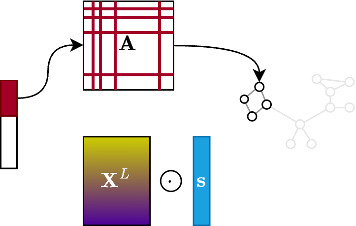

The $\texttt{CON}$ operation selects the columns and rows of the kept nodes.

The $\texttt{RED}$ operation, instead, takes the features of the top-K selected nodes and multiply them by the score vector to enable gradient flowing:

\[\mathbf{X}' = \left( \mathbf{X}^L \odot \sigma(\mathbf{s}) \right)_{\mathbf{i},:}\]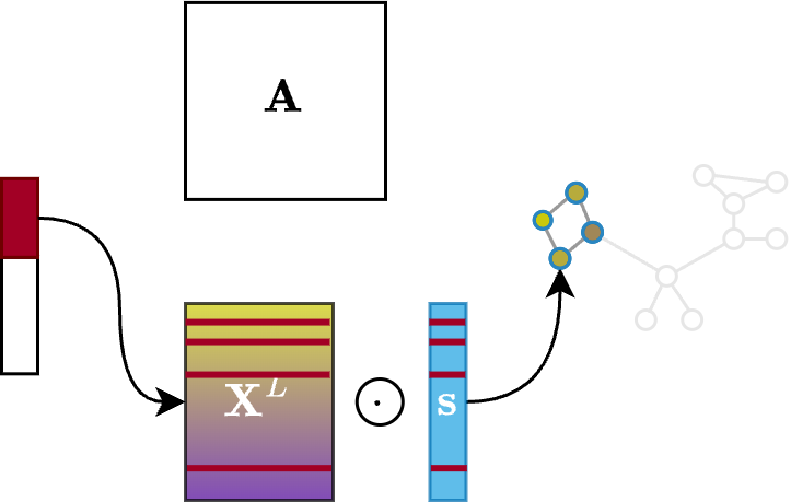

The $\texttt{RED}$ operation applies a sort of gating mechanism to the features of the pooled nodes to let gradients flow past the top-*K* operation.

What we just saw is the vanilla top-K pooling operator, that was introduced in the Graph U-Net paper[ûnet] as part of an architecture for node classification (very similar to the one we saw before). Many other score-based pooling methods were proposed afterwards. Most of them share the same basic idea and mainly differ in how they compute the score vector $\mathbf{s}$. In particular, they use more elaborated operations than just projecting the features with a vector $\mathbf{p}$.

Node selection and training

Something very peculiar of the score based pooling operators is that they tend to select as the supernodes of the pooled graph nodes that are very similar and nearby on the original graph. The reason is that after applying a stack of $L$ MP layers, nodes that are neighbors on the graph end up having very similar features. Since the score vector is obtained directly from those features, neighboring nodes will also have a similar score, meaning that the top-K nodes will come from the same part of the graph.

Note
Score-based methods keep only those nodes coming from the same part of the graph.

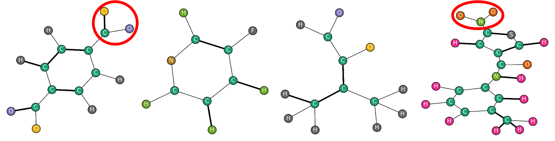
Clearly, this kind of pooling is quite restrictive because the pooled graph only keeps information about a limited portion of the original graph. If the downstream task requires to maintain information about the whole graph using these kind of pooling operation will not work well. So, when is that score-based pooling works? For example when the class of the graph depends only on a small piece of the whole graph, e.g., a specific motif whose presence or absence determines the class. These kind of examples can be found bio-informatics, where a property of a molecule is determined by the presence or the absence of a specific group of atoms. In those cases, a score based pooling operator can effectively isolate the relevant chunk of the graph and facilitate the retrieval of the relevant information.

In some tasks the class of the graph is determined by the presence of a particular motif in the graph. For example, the property of a molecule graph can be determined by the presence of a specific atomic structure.

Training a GNN with a score based pooler is generally faster and less memory demanding than using soft clustering pooling methods, but less efficient than using one-over-K methods, since the pooling operator comes with additional parameters (the projector $\mathbf{p}$).

Training of a GNN for graph-level tasks with score-based pooling layers.

Pros and Cons

To wrap up, score-based methods generally have the following pros and cons.

Pros:

✅ Offer some flexibility since the score vector $\mathbf{s}$ is influenced by the node features and the downstream task at hand.

✅ Have fewer parameters and lower computational complexity than soft clustering methods.

Cons:

❌ Completely discard some parts of the graph, which gives bad performance in tasks where preserving the whole graph structure, or simply different parts of the graph, matters.

At this point, it should be clear that there are profound differences between the different families of graph pooling operators. In the next part, we will discuss some strategies that allows us to select the most suitable approach.

📝 Citation

If you found this useful and want to cite it in your research, you can use the following bibtex.

@misc{bianchi2024intropool
  author = {Filippo Maria Bianchi},
  title = {An introduction to pooling in GNNs},
  year = {2025},
  howpublished = {\url{https://filippomb.github.io/blogs/gnn-pool-1/}}
}

Part 2

❹ Soft clustering pooling methods

Degenerate solutions

Auxiliary Losses

Pros and Cons

❺ One-over-K pooling methods

Graclus

Node Decimation Pool

k-Maximal Independent Sets

Pros and Cons

❻ Score-based pooling methods

Node selection and training

Pros and Cons

📚 References