Pooling in Graph Neural Networks (3/3)

This post is divided in three parts:

In the previous part, I introduced the different families of graph pooling operators, highlighting their respective strengths and weaknesses. In this part, I’ll discuss different approaches to evaluate their performance.

Part 3

❼ Evaluation procedures

At this point, we saw some of the main approaches to perform graph pooling and noticed that they are quite different in how they work and in the result they produce.

So, the next big question is:

Which pooling method should we use?

Answering this question is not trivial. In some cases, the nature of the data and the downstream task at hand can help us to take a more informed decision about which approach should be used. In other cases, however, the only way to find out is to give it a shot and see how a given method performs empirically. Which brings us to the next fundamental question:

How to measure the performance of a pooling operator?

Once again, this is not an easy question to answer. There exist different methods, but they measure different quantities and types of performance. Understanding them is important to realize what is going on and to make informed decisions.

Let’s see these approaches in detail.

Note
Which pooler to choose usually depends on the data, the resources, and the task at hand.

Raw performance on the downstream task

Clearly, the most straightforward approach is to equip a GNN with different pooling methods and see how it performs on a downstream task such as graph classification, graph regression, node classification, and so on. By looking, for example, at the different classification accuracies achieved, one could rank and select the pooling operators. Since this is intuitive and straightforward, this type of evaluation is the most popular in the literature. Thanks to their flexibility and capability to adapt well to the data and the task at hand, soft clustering methods usually achieve the best performance on several downstream task¹. So, if memory and computational constraints are not an issues, equipping a GNN with these pooling methods is usually a good idea.

However, evaluating a pooling operator directly on the downstream task is very empirical and, most importantly, indirect. In some cases it is difficult to disentangle the effect of the pooling operator from the other GNN components, its capacity, the training scheme, and so on. In fact, it would be perfectly reasonable to ask ourselves if the same pooling operator would have performed better if inserted within a different GNN architecture or used in a different downstream task or with different data. Also, if one method is performing good or bad we might want to understand better what is going on and how to improve the design of our model.

To answer these questions, let us consider two additional performance measures presented in the original SRC paper².

Preserving node information

The first approach focuses on evaluating how well the information contained in the vertices of the original graph is preserved in the pooled graph. Ideally, we would like a pooling operator to embed as much as possible of the original information in the pooled graph. If that is the case, most of the original information can be restored from it.

To measure this property, we can use an AutoEncoder architecture that tries to reconstruct the original node features $\mathbf{X}$ from those of the pooled graph $\mathbf{X}’$. Let $\tilde{\mathbf{X}}$ be the reconstructed features, we train the graph Autoencoder by minimizing the following reconstruction loss

\[\mathcal{L}_\text{rec} = \| \mathbf{X} - \tilde{\mathbf{X}} \|^2\]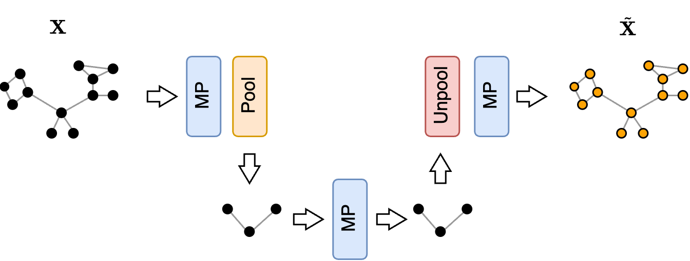

GNN architecture to evaluate the ability of a pooling method to preserve information from the original graph. The features of the original and reconstructed graph should be as similar as possible.

To see how this work in practice with different pooling operators let’s consider a set of point cloud graphs, where the node features are the coordinates of each point. If a pooling method manages to preserve most of the information in the pooled graph, the reconstructed point cloud should look similar to the original one.

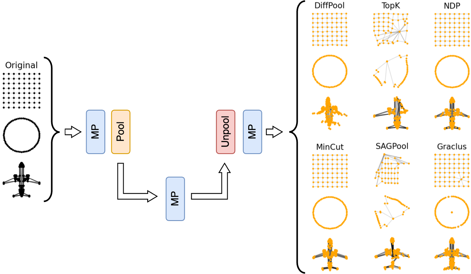
Original and reconstructed point cloud graphs when using six different pooling operators.

From this example we see that one-over-K methods such as NDP³ performs particularly well. On the other hand, we clearly see the main limitation of score-based method such as the vanilla top-K pooler⁴ and SAGPool⁵ that, by keeping only nodes from the same part of the graph, they fail to reconstruct the other sections.

Preserving topology

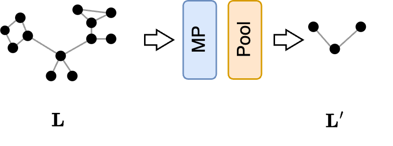
Next, we might be interested in seeing how much the topology of the pooled graph resembles the topology of the original graph. Since the two graphs have different sizes, comparing directly the elements of the adjacency matrices $\mathbf{A}$ and $\mathbf{A}’$ is not possible. However, it is possible to compare the spectrum (i.e., the eigenvalues) of their Laplacians, which should be as similar as possible. To encourage the spectra of the original and pooled graph to become similar, we can train a GNN to maximize the spectral similarity between the original and the pooled Laplacians⁶. The spectral similarity is a measure that compares the first $D$ eigenvalues of the two Laplacians $\mathbf{L}$ and $\mathbf{L}’$ and a loss that maximizes it can be defined as follows:

\[\mathcal{L}_\text{struct} = \sum_{i=0}^D \|\mathbf{X}_{:,i}^\top \mathbf{L} \mathbf{X}_{:,i} - \mathbf{X}_{:,i}^{'\top} \mathbf{L}' \mathbf{X}'_{:,i}\|^2\]

where $\mathbf{X}_ {:,i}$ and $\mathbf{X}’_{:,i}$ is the $i$-th eigenvector of $\mathbf{L}$ and $\mathbf{L}’$, respectively. The GNN architecture used in this task is very simple and consists just of a stack of MP layers followed by a pooling layer.

GNN architecture used to evaluate the ability of a pooling method to preserve in the pooled graph the same structure of the original graph.

Once the GNN is trained trained, we can compare the original and the pooled graphs and the adjacency matrices $\mathbf{A}$ and $\mathbf{A}’$ to see how similar they are.

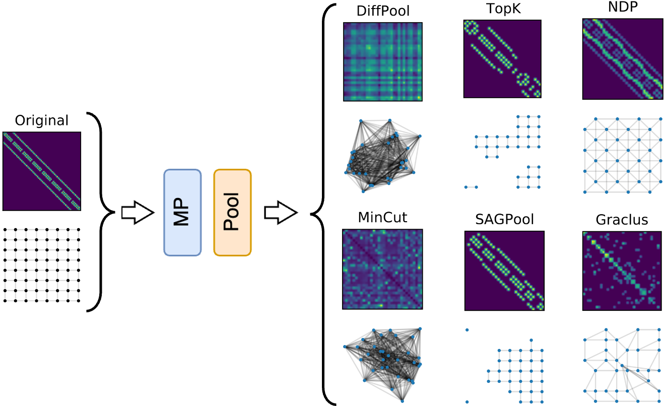
Adjacency matrix and structure of the original and pooled graph when using different pooling operators.

The examples in the figure show that soft clustering methods produce pooled graphs that are very dense and, even if informative, they have a structure that do not resemble at all the one of the original graph. On the other hand, since one-over-K methods perform a regular subsampling of the graph topology the structure of the pooled graph closely resemble that of the original graph. Finally, a regular structure like the grid is very similar to any of its subparts, meaning that the pooled graph obtained by score-based methods has a spectrum very similar to the original graph. Note that this is generally not true in graphs with less regular structures, where the overall spectrum is different from the one of the subgraphs.

Expressiveness

All the performance measures we saw so far are rather empirical and provide a quantitative result. There is, however, a theoretical result that allows us to measure the performance of a pooling method from a qualitative perspective in terms of its expressive power ⁷. The result can be summarized as follows.

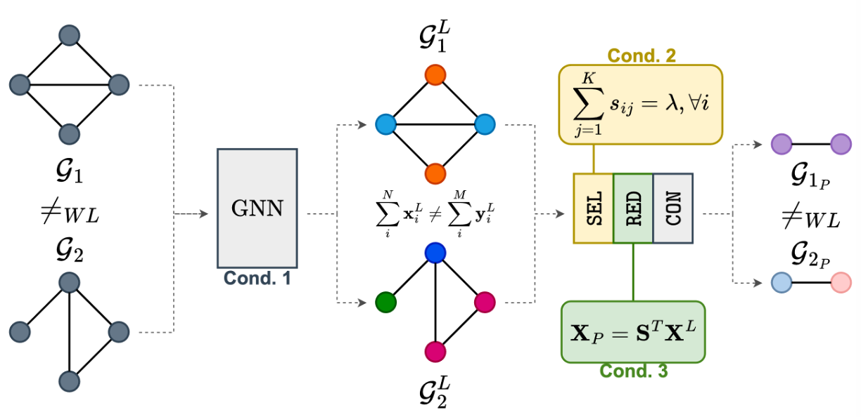
Given two graphs $\mathcal{G}_ 1$ and $\mathcal{G}_ 2$ that are different and that can be distinguished by a test for isomorphism called “WL test”, a pooling operator is expressive if the pooled graphs $\mathcal{G}_ {1_ P}$ and $\mathcal{G}_ {2_ P}$ can still be distinguished.

The conditions for expressiveness are three and are relatively easy to check.

The GNN part before the pooling layer must be expressive itself. To be sure that this is the case, it is enough to use expressive MP layer such as GIN⁸. This ensures that the node features $\mathbf{X}^L$ and $\mathbf{Y}^L$ associated with the two graphs $\mathcal{G}_1^L$ and $\mathcal{G}_2^L$ after applying $L$ MP layers are different, i.e., $\sum_i^N \mathbf{x}_i^L \neq \sum_i^M \mathbf{y}_i^L$ , where $N$ and $M$ are the number of vertices in the two graphs.
The $\texttt{SEL}$ operation must be such that all nodes in the original graph are included in at least one supernode of the pooled graph. This condition can be conveniently checked by considering an association matrix $\mathbf{S} \in \mathbb{R}^{N \times K}$, analog to the one we saw in the soft clustering methods, that maps each node of the original graph to the nodes of the pooled graph. If the elements in each row of $\mathbf{S}$ sum to a constant value, i.e., if $\sum_{j=1}^K s_{ij} = \lambda$, then each node from the original graph is represented in the pooled graph.
The $\texttt{RED}$ operation must ensure that the features of the pooled nodes $\mathbf{X}_P$ (or $\mathbf{X}’$, as we called them before), are a weighted combination of the original features and the weights should be given by the membership values in $\mathbf{S}$ . This happens when $\mathbf{X}’ = \mathbf{S}^\top \mathbf{X}$.

A GNN with expressive MP layers (condition 1) computes different features for graphs that are WL-distinguishable. A pooling layer satisfying the conditions 2 and 3 generates coarsened graphs that are still distinguishable.

If we look back at the definition of soft clustering method, we can easily see that they all satisfy condition 2 and 3 meaning that they are expressive. On the other hand, in score-based methods the rows of $\mathbf{S}$ associated with the dropped nodes are zero, because they are not assigned to any supernode. As such, score-based poolers are not expressive, meaning that it might be no longer possible to distinguish their pooled graphs even if the original graphs were different. For one-over-K methods the situation is a bit more complicated. Some methods like NDP are not expressive because they drop the nodes of one side of the MAXCUT partition. Other methods like k-MIS are expressive because they assign all nodes to those in the maximal independent set.

An important remark is that the three conditions above are sufficient but not necessary. This means that an expressive pooling operator always creates pooled graph that are distinguishable if the original ones were distinguishable. However, there could also be a non-expressive pooling operator that produces distinguishable pooled graphs.

❽ Concluding remarks

Let’s recap what we’ve covered in these posts.

In Part 1, we introduced Graph Neural Networks (GNNs) and graph pooling through an analogy with the more intuitive—and arguably simpler—Convolutional Neural Networks (CNNs) used in computer vision. Then, we presented a general framework called Select-Reduce-Connect (SRC), which provides a formal definition of graph pooling and unifies many different pooling approaches under one umbrella.

In Part 2, we explored three different families of graph pooling methods: soft clustering, one-over-K, and score-based approaches. We reviewed key representatives of each family and demonstrated how they can be expressed within the SRC framework. For each family, we highlighted their main pros and cons.

In Part 3, we examined how to evaluate a pooling operator using three quantitative measures: its performance on downstream tasks, its ability to preserve information from the original graph, and the similarity between the spectra of the original and pooled graphs. We also discussed a theoretical measure that characterizes a pooling operator qualitatively based on its expressiveness—that is, its ability to preserve the distinguishability of the original graphs in the pooled graphs.

Graph pooling software library

While libraries such as PyTorch Geometric and Spektral come with several pooling operators already implemented, they lack more recent approaches and do not provide a unified API for the different pooling operators.

Here enters Torch Geometric Pool (🎱 tgp), the first library explicitly made for pooling in GNNs.

Explicitly designed for PyTorch Geometric, 🎱 tgp implements every pooling operator according to the SRC framework. Each pooling layer in 🎱 tgp can be just dropped into a GNN architecture implemented in PyTorch Geometric, without making any major change to the original architecture or to the training procedure, making it very easy to build a GNN with hierarchical pooling. Check out the tutorials page to learn how to use 🎱 tgp at its best, how to quickly deploy existing pooling operators, and how to design new ones!

Open challenges

I hope this introduction has shed some light on this fascinating research area. There are many other graph pooling approaches that I did not cover in this post, and they are out there for you to discover. Given the variety and diversity of existing methods and the overall complexity of graph pooling, there are still many open possibilities for crafting new and more efficient pooling operators that can overcome some limitations of the current ones.

Key open research areas include improving the scalability of soft clustering methods and enabling them to learn pooled graphs of varying sizes. Additionally, there’s the challenge of eliminating the top-K selection in score-based methods—which is not differentiable—while preserving their scalability, and selecting supernodes in a more uniform manner, similar to one-over-K methods. Interestingly, the different families of pooling operators are complementary in terms of strengths and weaknesses, suggesting that the next generation of pooling operators could combine their strengths to harness the best of all worlds.

I hope you enjoyed this post and that I have piqued your interest in graph pooling.

📝 Citation

If you found this useful and want to cite it in your research, you can use the following bibtex.

@misc{bianchi2024intropool
  author = {Filippo Maria Bianchi},
  title = {An introduction to pooling in GNNs},
  year = {2025},
  howpublished = {\url{https://filippomb.github.io/blogs/gnn-pool-1/}}
}