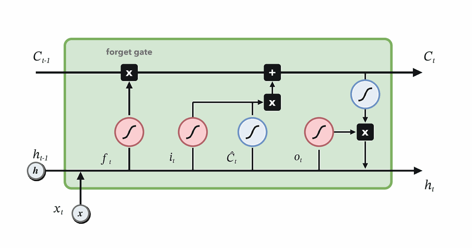
Forget gate
Decide which parts of the previous memory survive.
\(f_t = \sigma(W_f[h_{t-1}, x_t] + b_f)\)
\(f_t \odot C_{t-1}\)
How neural networks represent the past.
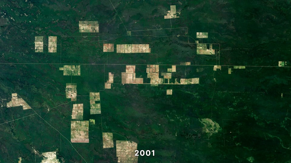
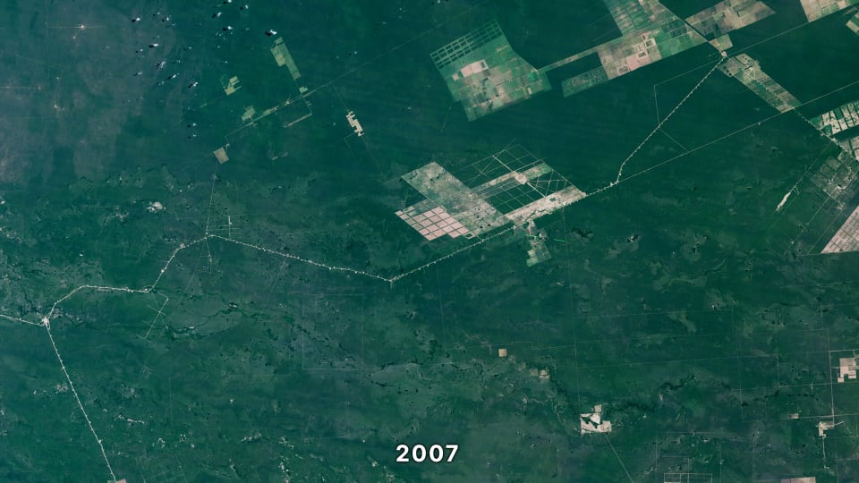
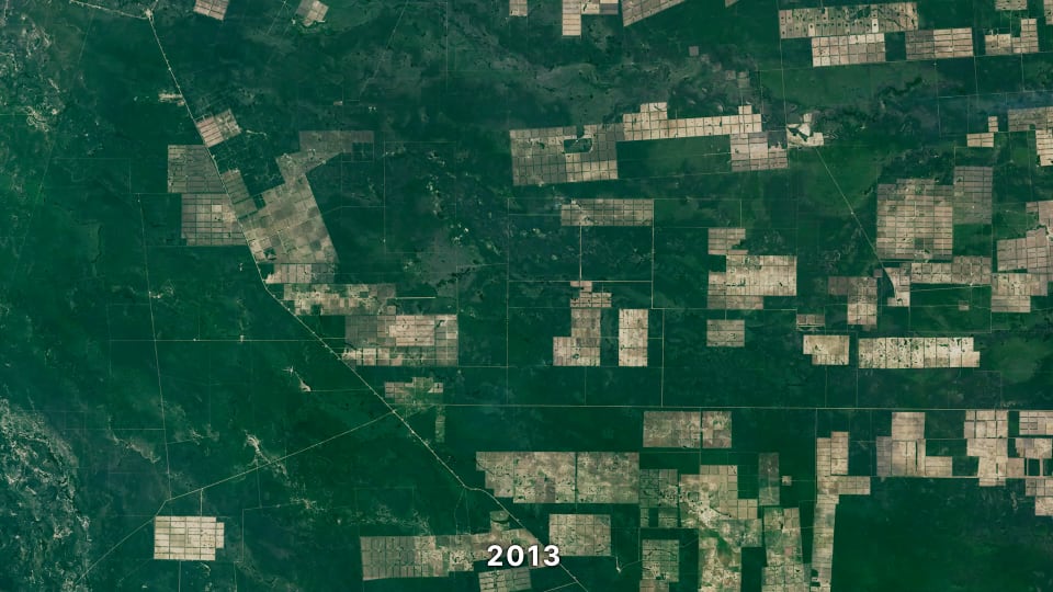
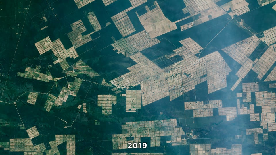
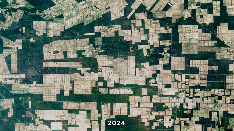
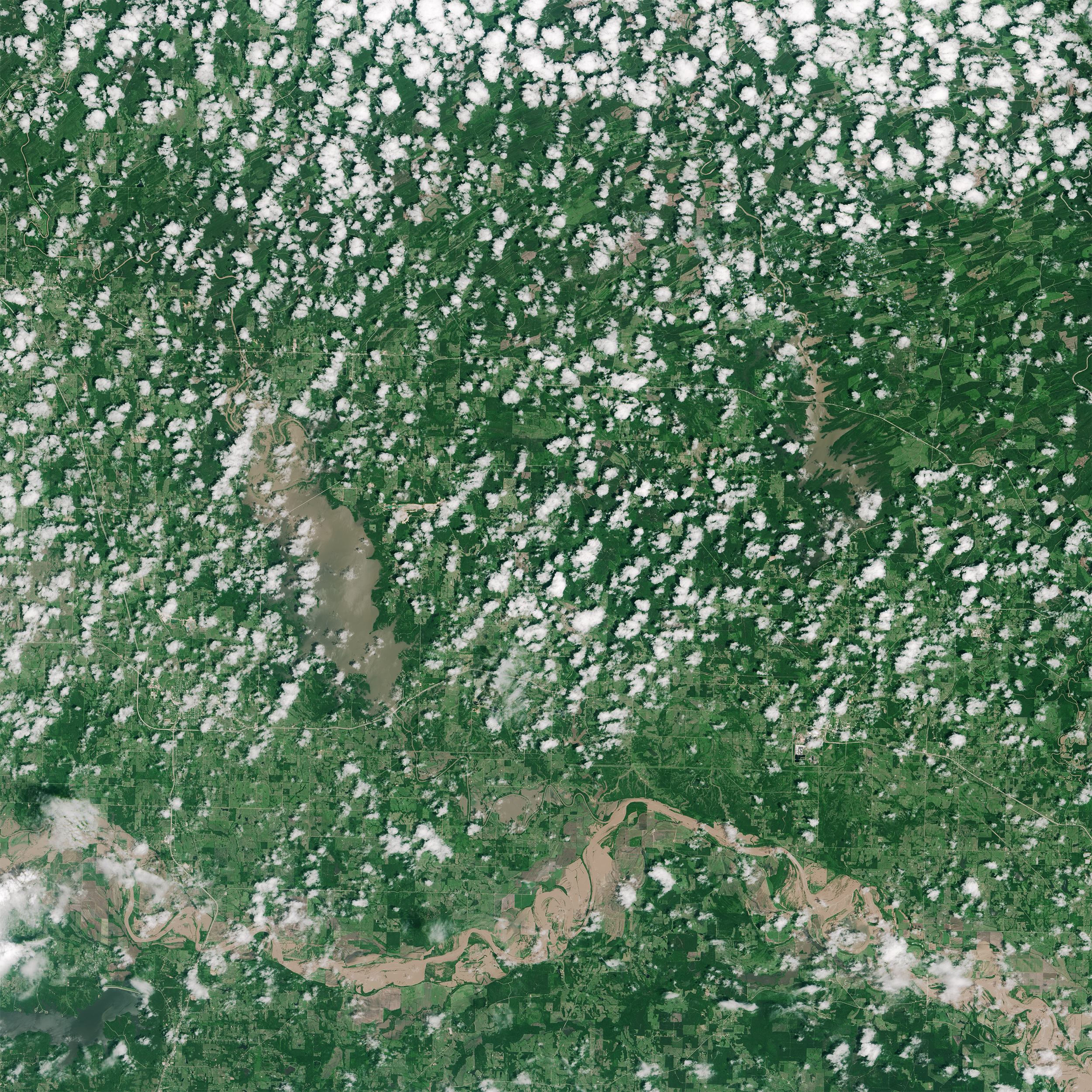
NASA Landsat Science, "Chaco Region Paraguay Time Series", 2025.
Normalized Difference Vegetation Index (NDVI) quantifies vegetation by measuring the difference between near-infrared (which vegetation strongly reflects) and red light (which vegetation absorbs).
NDVI time series reveal vegetation dynamics that single images miss.
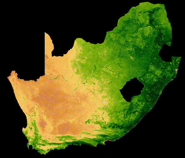
NDVI change over South Africa across a single year.
NDVI context adapted from White, Introduction to Spatial Data in R, 2022.
Before: March 23, 2015
After: May 26, 2015
NASA Earth Observatory images by Joshua Stevens, using Landsat data from the U.S. Geological Survey.
Load consumption profile on a backbone of the electricity network of Rome. The temperature-load relation is nonlinear; copying yesterday is the first baseline to beat.

Bianchi et al., "Recurrent neural networks for short-term load forecasting: an overview and comparative analysis", 2017.
The signal is often not in one observation, but in how observations change.
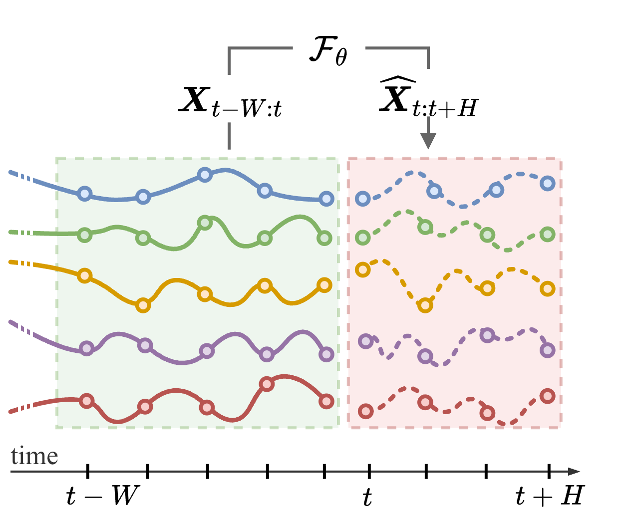
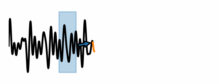
Past context is useful only relative to a prediction horizon.
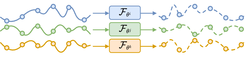
Tailored, data inefficient.
\(\widehat{X}^{\,i}_{t:t+H}=\mathcal{F}_{\theta^i}(X^{\,i}_{t-W:t})\)
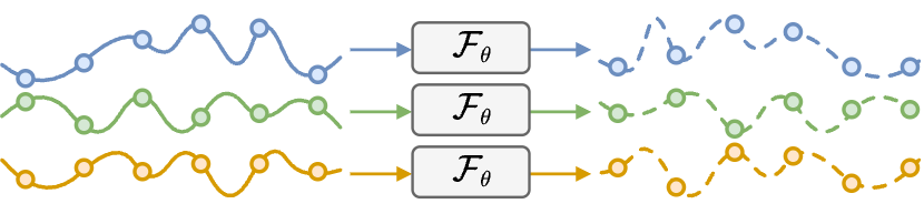
Shared, scalable.
\(\widehat{X}^{\,i}_{t:t+H}=\mathcal{F}_{\theta}(X^{\,i}_{t-W:t}, a^{\,i})\)
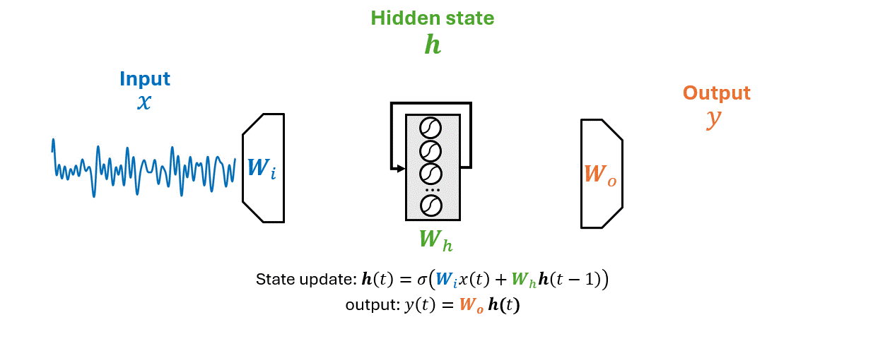
How should the model represent the past?
Cini et al., "Graph Deep Learning for Spatiotemporal Time Series", 2023.
Bianchi, Time Series Analysis with Python, online handbook, 2024.
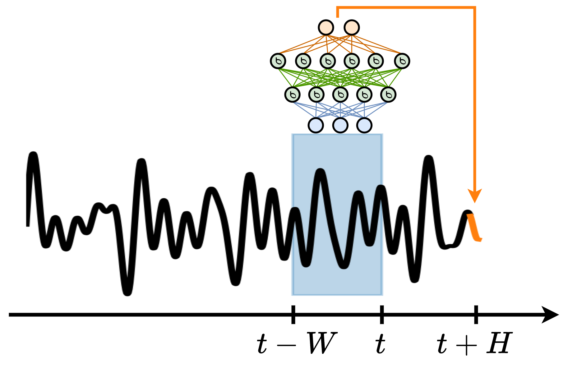

Can the model learn its own memory?
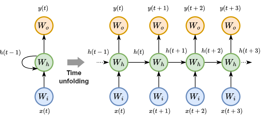
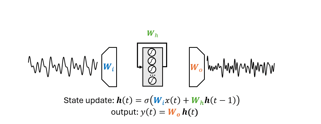
Vanishing and exploding gradients make the training of RNNs challenging.
Decide which parts of the previous memory survive.
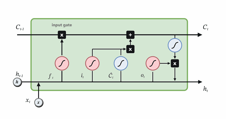
Choose how much new candidate content to write.
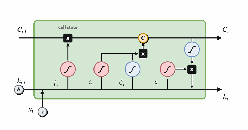
Combine retained and written memory, then expose useful state.
Hochreiter and Schmidhuber, "Long short-term memory", 1997.
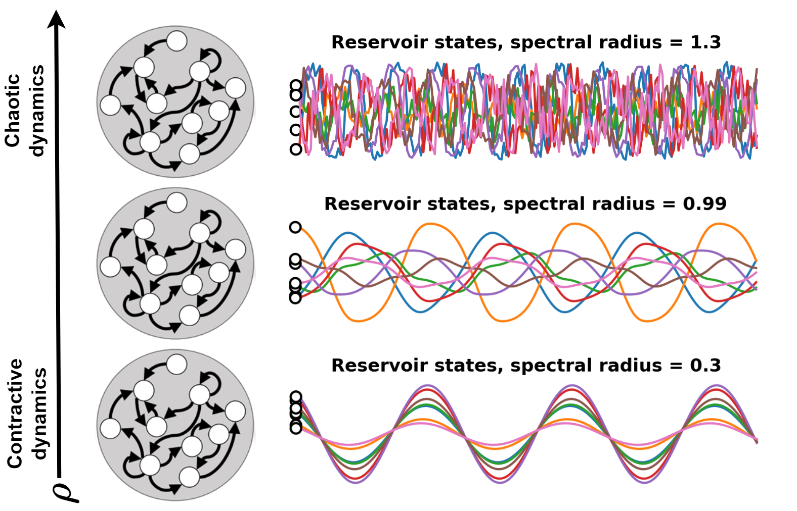
Useful when training a standard RNN is too expensive or when data are not enough.
Bianchi et al., "Reservoir computing approaches for representation and classification of multivariate time series", 2020.
A small kernel scans space and reuses the same detector at every location.
The same learned kernel scans time to detect slopes, peaks, pulses, or changes.
The same learned kernel is applied at every time step.
A TCN grows memory by composing small filters across layers.
The receptive field is the maximum history that can affect one output.
For forecasting, every output must ignore observations from the future.
Preprocessing, normalization, and imputation must also respect time.
Van Den Oord et al., "Wavenet: A generative model for raw audio", 2016.
A temporal CNN acts learns a bank of filters matching temporal patterns.
Good fit when local temporal shapes are informative and transferable across locations.
Each token asks which other observations are relevant.
Attention selects observations by content; time encodings tell it when they occurred.
Vaswani et al., "Attention Is All You Need", 2017.
A temporal Transformer does not only need observations. It also needs to know when they happened and whether they should be used.
The model ignores unavailable dates and can focus attention on the most informative ones.
Instead of storing a finite window, model a hidden state that evolves in continuous time.
Continuous dynamics evolve across irregular gaps; updates happen at observation times.
Chen et al., "Neural Ordinary Differential Equations", 2018; Rubanova et al., "Latent ODEs for Irregularly-Sampled Time Series", 2019.
Observe the continuous system only at times \(t_i\).
The elapsed time
\(\Delta t_i=t_i-t_{i-1}\) determines how far the state evolves.
After discretization, the sequence is processed by scanning \(s_0 \rightarrow s_1 \rightarrow \cdots\).
\(A,B,C,D\) define state dynamics, input injection, readout, and skip connection; the layer learns these dynamics.
Gu et al., "Combining recurrent, convolutional, and continuous-time models with linear state space layers", 2021.
All state-space models carry a compact hidden state. S4 makes this efficient for long sequences; Mamba makes it selective.
S4: Gu, Goel, and Ré, 2021. Mamba: Gu and Dao, 2023.
| Architecture | Memory mechanism | Parallelism | Good fit | Watch out |
|---|---|---|---|---|
| Window + MLP | Fixed explicit lags | High | Baselines; engineered features | Choosing window size \(W\) |
| RNN/GRU/LSTM | Learned recurrent state | Low across time | Streaming prediction; regime/state tracking | Difficult and expensive training |
| Reservoir/ESN | Random dynamical features | Medium | Limited labels; fast readouts | Sensitive hyperparameters' tuning |
| TCN | Receptive field by depth/dilation | High | Recurring patterns; local motifs | Context by design |
| Transformer | Direct attention over observed dates | High | Arbitrary temporal interactions; masked gaps | Memory cost |
| SSM/Mamba | Structured state-space scan; input-selective updates | High / streaming | Very long sequences; efficient streaming context | Newer ecosystem |