AR-MA#

Overview#
In this lecture we will cover:
The autocorrelation function (ACF).
The partial autocorrelation function (PACF).
Explanation of how autoregressive and moving average models work.
Correlations in time series#
The correlation function measures the degree of association between two random variables.
In time series data it measures the association btween two different points in time.
Correlation is essential for understanding the linear relationship and dependency in time series data.
There are two types of correlation functions:
Autocorrelation.
Cross-Correlation.
Autocorrelation Function (ACF)#
The ACF measures the correlation of a time series with its own lagged values
where:
\(k\) is the lag number.
\(X(t)\) is the value at time \(t\).
\(\mu\) is the mean of the series.
\(\sigma^2\) is the variance of the series.
Values close to 1 or -1 indicate strong correlation, while values near 0 indicate weak correlation.
n = 100
time_series_1 = np.random.normal(0, 0.5, n) + np.sin(2*np.pi/10*np.arange(n))
fig, axes = plt.subplots(1, 2, figsize=(12, 3))
axes[0].plot(time_series_1)
axes[0].set_title('Original Time Series')
plot_acf(time_series_1, lags=20, alpha=0.05, ax=axes[1]); # We plot the first 20 lags. We could plot more by changing the `lags` argument.
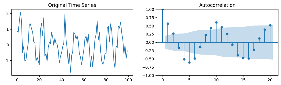
The stems represent lagged correlation values.
The time series correlates well with itself shifted by 1 (lag 1).
A lag of 2 correlates nearly but not quite as well. And so on.
The blue region represents a confidence interval.
Correlations outside of the confidence interval are statistically significant whereas the others are not.
\(\alpha\) in this case was 0.05 (95% confidence interval), but it can be set to other levels.
See the the documentation for more details.
Cross-Correlation Function (CCF)#
CCF measures the correlation between two time series at different lags:
where:
\(X\) and \(Y\) are two different time series.
\(\mu_x, \mu_y\) are their means, and \(\sigma_x, \sigma_y\) are their standard deviations.
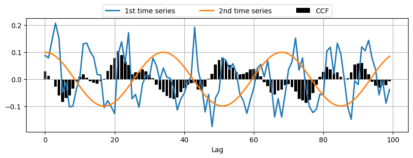
The CCF is commonly used for searching a shorter, known feature, within a long signal.
time_series_2 = np.cos(np.pi/17*np.arange(n))

# Calculate CCF between the two time series
ccf_vals = ccf(time_series_1, time_series_2, adjusted=False)

# Plot CCF
_, ax = plt.subplots(1,1,figsize=(10,3))
ax.bar(range(len(ccf_vals)), ccf_vals, color='k', label='CCF')
ax.plot(time_series_1*0.1, linewidth=2, label='1st time series')
ax.plot(time_series_2*0.1, linewidth=2, label='2nd time series')
plt.xlabel('Lag')
plt.legend(bbox_to_anchor=(0.2, 1.01, .6, 1.5), loc='lower center', ncol=3, mode="expand", borderaxespad=0.)
plt.grid();
Practical Applications of Correlation Functions
Identifying the nature of the data (e.g., whether it is random, has a trend or a seasonality).
Helping to determine the order of ARIMA models (more on this later on).
Identifying outliers in time series data.
Limitations and Considerations#
Correlation functions only measure linear relationships.
For meaningful results, time series should be stationary.
High correlation does not imply causation and can sometimes be misleading.

ACF measures both direct and indirect correlations between lags.
A strong correlation at higher lags could be a result of the accumulation of correlations at shorter lags.
Consider for example a random walk:
You may think that only lag \(h=1\) is important, but…
random_walk = np.cumsum(np.random.normal(0, 1, 100))

fig, axes = plt.subplots(1, 2, figsize=(12, 4))
axes[0].plot(random_walk)
axes[0].set_title('Random Walk')
plot_acf(random_walk, lags=20, alpha=0.05, ax=axes[1])
axes[1].set_title('Autocorrelation of Random Walk')
plt.tight_layout()
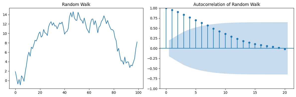
You can see that lags \(h>1\) are also present in the ACF.
Those are indirect correlations due to the accumulation of the main correlation at lag \(h=1\).
The Partial Autocorrelation Function (PACF)#
PACF addresses the 4th limitation of ACF by isolating the direct correlation between a time series and its lagged version.
It does that by removing the influence of correlations at shorter lags.
High PACF at lag \(k\) indicates a strong partial correlation with the \(k\)-th lag, not accounted for by correlations at lower lags.
PACF of lag \(k\) is sometimes denoted as \(\phi_{kk}\):
where:
\(\hat{X}(t)\) is the predicted value of \(X(t)\) based on all the values up to \(t-1\).
\(\hat{X}(t-k)\) is the predicted value of \(X(t-k)\) based on all the values up to \(t-k-1\).
Using ACF and PACF together provides a more comprehensive understanding of the time series data.
ACF helps in identifying the overall correlation structure and potential seasonality.
PACF pinpoints the specific lags that have a significant direct impact on the current value.
Example
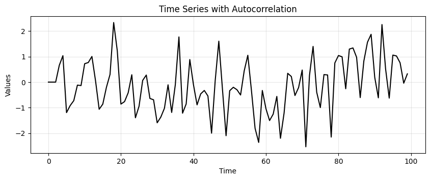
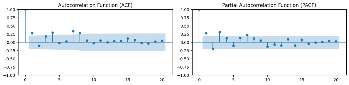
Consider a time series where ACF shows significant correlation at lags 1, 2, and 3.
Without PACF, it is unclear whether the correlation at lag 3 is direct or merely a reflection of the strong correlations at lags 1 and 2.
PACF can clarify this by showing whether there is a significant direct correlation at lag 3.
n = 100
time_series = np.zeros(n)
alpha1, alpha2, alpha3 = 0.6, -0.3, 0.2  # Coefficients to induce autocorrelation at lags 1, 2, and 3
noise = np.random.normal(0, 1, n)

# Generate correlated data
for t in range(3, n):
    time_series[t] = alpha1 * time_series[t-1] + alpha2 * time_series[t-2] + alpha3 * time_series[t-3] + noise[t]
run_sequence_plot(np.arange(100), time_series, title='Time Series with Autocorrelation');
_, (ax1, ax2) = plt.subplots(1, 2, figsize=(12, 3))

# Plot ACF
plot_acf(time_series, ax=ax1)
ax1.set_title('Autocorrelation Function (ACF)')

# Plot PACF
plot_pacf(time_series, ax=ax2)
ax2.set_title('Partial Autocorrelation Function (PACF)')
plt.tight_layout()
Lag estimation with ACF and PACF is helpful in modelling time-series with autoregressive and moving-average models that we’ll introduce in the next sections.
Autoregressive (AR) models#
An Autoregressive (AR) model is a type of time series model that uses observations from previous time steps as input to a regression equation to predict the value at the next time step.
The AR model is dependent solely on its own past values.
The general form of an AR model of order \(p\) is:
where
\(X(t)\): Time series value at time \(t\).
\(c\): Constant term (also known as the intercept).
\(\phi_1, \phi_2, \dots, \phi_p\): Coefficients of the model.
\(p\): Order of the AR model (number of lag terms).
\(\epsilon_t\): Error term (white noise) at time \(t\).
AR(1) Model
The first-order autoregressive model, AR(1), is
In an AR(1) model, the current value is based on the immediately preceding value.
Example: A simple stock price model where today’s price is partially dependent on yesterday’s price.
Higher Order AR Models
Higher order AR models (AR(2), AR(3), etc.) depend on more than one past value.
For example, the AR(2) model is:
These models are useful in scenarios where the effect of more than one previous time step is significant.
Estimating AR Model Coefficients
Coefficients of AR models can be estimated using various methods like the Maximum Likelihood Estimation, or Least Squares Estimation.
The estimated coefficients provide insights into the influence of past values on the current value in the time series.
In other words, AR models are interpretable.
Limitations of AR Models
AR models require the time series to be stationary.
Higher order AR models can overfit the training data and perform bad in prediction.
They cannot model non-linear relationships in the data.
Natively, the AR models do not account for exogenous factors.
These, usually are additional time series that are relevant for the prediction.
For example, the time series of the temperatures when predicting the electricity load.
There are extensions (ARMAX) that allow to include exogenous variables in the model.
AR model identification#
How do we determine the correct order \(p\) of the AR model?
We do that by looking at the first lags of the PACF.
Let’s see it through an example.
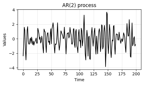
We generate some data from an AR(2) process with coefficients
[1.0, -0.5, 0.7].Note that the
1.0at the beginning refers to the zero-lag and is always1.0.
ar_data = arma_generate_sample(ar=np.array([1.0, -0.5, 0.7]), ma=np.array([1]), nsample=200, scale=1, burnin=1000)
_, ax = plt.subplots(1, 1, figsize=(5, 3))
run_sequence_plot(np.arange(200), ar_data, ax=ax, title="AR(2) process")
plt.tight_layout()
_, ax = plt.subplots(1, 1, figsize=(5, 3))
plot_acf(ar_data, ax=ax, title="ACF of the AR process")
plt.tight_layout();
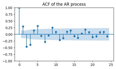
The actual coefficients of the AR(2) process are not clearly visible in the ACF plot.
Next, we compute the PACF on the
ar_data.
_, ax = plt.subplots(1, 1, figsize=(5, 3))
plot_pacf(ar_data, ax=ax, title="PACF of the AR process")
plt.tight_layout();
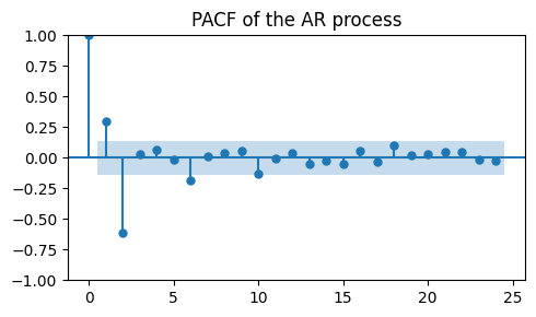
Besides the spike at lag 0, which is always there, we see two significant lags:
The positive spike at lag 1, introduced by the negative coefficient
-0.5.The negative spike at lag 2, introduced by the positive coefficient
0.7.
This means that the process has a memory of length 2.
In other words, (most of) the correlations in the data are explained by the previous 2 time steps.
If we want to fit an AR model to our data we would choose \(p=2\), which is a AR(2) model.
Finally, an AR process is characterized by correlations that decay slowly in time.
This can be seen by looking at the ACF plot, where we see significant spikes over many lags.
_, ax = plt.subplots(1, 1, figsize=(5, 3))
plot_acf(ar_data, ax=ax, title="ACF of the AR process")
plt.tight_layout()
⚙ Try it yourself
Try modifying/adding/removing values in the
arcoefficients inarma_generate_sample.Then, see how the PACF plot changes.
Forecasting with AR models#
How do we compute forecasts using an AR model?
In general, our time series has a trend and a seasonality.
However, an AR model can only be used on stationary data.
Therefore, we need to do the following steps.
Step 1: Remove trend and seasonality
Before applying an AR model is necessary to make the time series stationary.
This can be done using techniques we saw in the previous chapters.
Two possibile ways of doing it are:
Apply standard and seasonal differencing to the time series.
\[\begin{split} \begin{aligned} R'(t) = X(t + 1) - X(t) & \qquad \text{removes trend} \\ R(t) = R'(t + L) - R'(t) & \qquad \text{removes seasonality} \end{aligned} \end{split}\]Estimate trend \(T\) and seasonality \(S\) (e.g., by using seasonal decomposition or smoothing techniques) and subtract them:
\[R(t) = X(t) - T(t) - S(t)\]
Step 2: Apply the AR model
Identify the order of the AR model.
Fit an AR model to the detrended and deseasonalized time series \(R(t)\).
Use the model to forecast the next values \(\hat R(t+h), h=1, \dots, H\) where \(H\) is the forecast horizon.
Step 3: Reconstruct the forecast
The reconstruction procedure depends on how we made the time series stationary at step 1.
If we used differencing:
We must undo the differentiation by taking cumulative sums of the residuals.
If we removed the trend and seasonality that we modelled, for each \(h \in [1, H]\) we must:
Predict the trend \(\hat{T}(t+h)\) and the seasonal component \(\hat{S}(t+h)\).
Add back the estimated trend and seasonality to the forecasted value:
\[\hat X(t+h) = \hat R(t+h) + \hat{T}(t+h) + \hat{S}(t+h)\]
Example: forecasting with AR model#
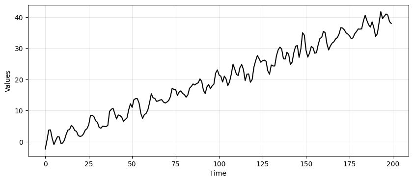
Let’s generate some data with trend and seasonality.
time = np.arange(200)
trend = time * 0.2
seasonality = 2*np.sin(2*np.pi*time/12) # Seasonality 12
time_series_ar = trend + seasonality + ar_data

_, ax = plt.subplots(1, 1, figsize=(10, 4))
run_sequence_plot(time, time_series_ar, "", ax=ax);
Since we are going to compute forecasts, let’s divide the data in a train and test set.
train_data_ar = time_series_ar[:164]
test_data_ar = time_series_ar[164:]
To determine the order \(p\) of the AR model we need to look at the PACF.
The order \(p\) corresponds to the least nonzero lag in the PACF plot.
_, ax = plt.subplots(1, 1, figsize=(5, 3))
plot_pacf(train_data_ar, ax=ax)
plt.tight_layout();
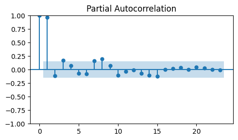
The PACF would suggest an order \(p=1\).
However, this PACF makes little sense.
As we discussed before, both the ACF and PACF should be computed on stationary data.
If data are stationary, correlations drop quickly.
If they don’t, that’s a sign that your data is not stationary.
Since we generated the time series by hand we know that it has trend and seasonality and, therefore, it is not stationary.
However, to be rigorous we’ll test the time series with the Augmented Dickey-Fuller (ADF) test.
_, pvalue, _, _, _, _ = adfuller(train_data_ar)
print(f"p-value: {pvalue:.3f}")
p-value: 0.833
Such a high \(p\)-value means that we fail to reject the null hypothesis
No surprises here.
To achieve stationarity we can transform the data by applying one of the techniques discussed in step 1.
Let’s first try with differencing.
Stationairty through differencing#
We start by applying 1st-order differencing to remove the trend.
Then, we check the stationarity of the differenced data with the ADF test.
diff_ar = train_data_ar[1:] - train_data_ar[:-1]

_, pvalue, _, _, _, _ = adfuller(diff_ar)
print(f"p-value: {pvalue:.3f}")
p-value: 0.000
The ADF test suggests that now the time series is stationary.
We might want to apply also seasonal differentiation to get rid of the seasonal component.
However, differencing too many times might compromise the structure of the data.
This problem is called overdifferencing.
See this explanation for how to determine the optimal order of differentiation.
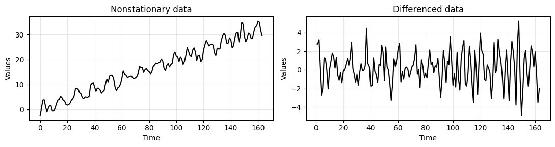
Let’s see how data looks like after 1st-oder differencing.
_, axes = plt.subplots(1,2, figsize=(11,3))
run_sequence_plot(time[:len(train_data_ar)], train_data_ar, title="Nonstationary data", ax=axes[0])
run_sequence_plot(time[1:len(train_data_ar)], diff_ar, title="Differenced data", ax=axes[1])
plt.tight_layout();
Let’s recompute the PACF on the differenced data.
We also compare it to the PACF on the original
ar_dataand the nonstationary datatrain_data_ar.
_, axes = plt.subplots(1, 3, figsize=(12, 3))
plot_pacf(ar_data[:len(train_data_ar)], ax=axes[0], title="PACF Original AR process")
plot_pacf(train_data_ar, ax=axes[1], title="PACF Nonstationary time series")
plot_pacf(diff_ar, ax=axes[2], title="PACF Differenced time series")
plt.tight_layout();
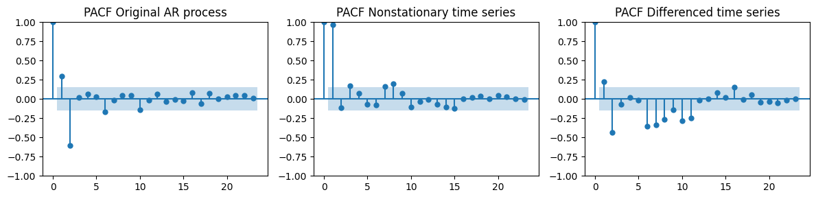
The prominent negative spike at lag 2 appears both in the PACF of the original AR data and in the differenced time series.
These two look way more similar than the PACF we got for the nonstationary data.
The prominent spike at lag 2 suggests that \(p=2\), i.e., we should use an AR(2) model.
Attention
In the differenced time series there are also other significant spikes at higher lags, which are not present in the original AR data.
This is because there is a seasonal component left in the data.
Let’s see if we can remove them by applying seasonal differencing and recompute the PACF plot.
# Seasonal differencing
diff_diff_ar = diff_ar[12:] - diff_ar[:-12]

_, ax = plt.subplots(1, 1, figsize=(5, 3))
plot_pacf(diff_diff_ar, ax=ax, title="PACF after 1st order and seasonal differencing")
plt.tight_layout();
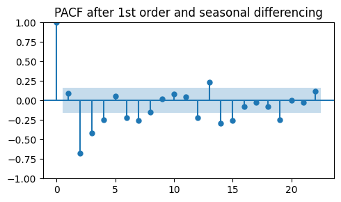
Even after seasonal differencing we are not able to recover the PACF of the original data.
On the contrary, this PACF looks even more different than the original one.
In practice, it is rare to get a “clean” PACF with only one prominent lag at the correct order when using differencing.
Interpreting the PACF (and ACF) plots to select the order of the model requires skills and experience.
See this guide for selecting the best AR (and MA) order.
Note
Besides overdifferencing, other issues appear when stationarity is achieved with differencing.
Some data are lost at the beginning or at the end of the time series due to differencing.
For example, when applying 1st order and seasonal differencing \(L+1\) steps are lost.
In addition, it is easy to make mistakes when reverting the differencing to make predictions.
This further complicates when there is a gap between the training and test set or when the forecast horizon \(H\) goes beyond the seasonality \(L\).
Note
Should we perform seasonal or 1st order differencing first?
Both paths are valid, however seasonal differencing is usually done first.
Often seasonal differeing is enough to make the data (almost) stationary.
In general, we want to do as little differencing as possible to avoid overdifferencing.
Stationarity by subtracting estimated trend and seasonality#
As an alternative approach, we can estimate the trend and seasonality with Triple exponential smoothing (TES).
Then, we compute the residuals subtracting the estimated trend and seasonality.
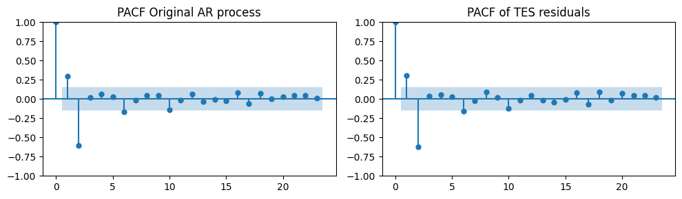
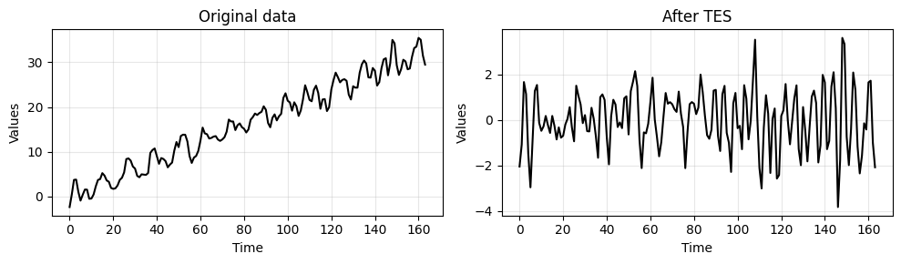
We see that, in this case, the residuals are much closer to our original AR process.
tes = ExponentialSmoothing(train_data_ar, trend='add',
                           seasonal='add', seasonal_periods=12).fit()
trend_and_seasonality = tes.fittedvalues # Estimated trend and seasonality
tes_resid = train_data_ar - trend_and_seasonality

_, axes = plt.subplots(1, 2, figsize=(10, 3))
plot_pacf(ar_data[:len(train_data_ar)], ax=axes[0], title="PACF Original AR process")
plot_pacf(tes_resid, ax=axes[1], title="PACF of TES residuals")
plt.tight_layout();
_, ax = plt.subplots(1, 2, figsize=(10, 3))
run_sequence_plot(time[:len(train_data_ar)], train_data_ar, title="Original data", ax=ax[0])
run_sequence_plot(time[:len(train_data_ar)], tes_resid, title="After TES", ax=ax[1])
plt.tight_layout()
Tip
In this case, we knew the main period to be
12.In general, we need to estimate it.
We can use the
fft_analysisfunction from Lecture 1.
from tsa_course.lecture1 import fft_analysis

period, _, _ =fft_analysis(time_series_ar)
print(f"Period: {np.round(period)}")
Period: 12.0
Attention
Smoothers work so well here because we use toy data with additive components, linear trend, constant variance, etc…
Many real-world data do not look so nice.
In some cases, we have to rely on other techniques, including differentiation and the “dirty” ACF/PACF plot we got from it.
Once the data are stationary, we are ready to fit the AR(2) model to make forecasts.
Depending on which method we used to obtain stationary data, we must do something different to reconstruct the predictions.
Let’s start with the stationary data obtained from differencing.
Predictions with differencing approach#
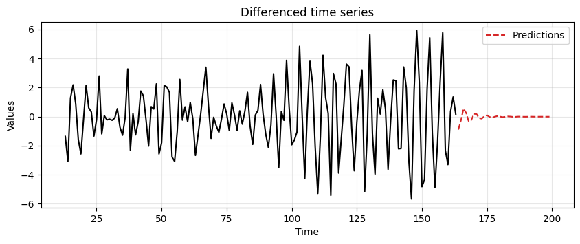
First, we use
diff_diff_arto fit an AR(2) model and make forecasts for a period as long as the test data.Note how after a short while the forecast goes to zero.
This, indicates that the AR(2) model is very uncertain about long-terms forecasts.
# Fit the model
model = ARIMA(diff_diff_ar, order=(2,0,0))
model_fit = model.fit()

# Compute predictions
diff_preds = model_fit.forecast(steps=len(test_data_ar))

ax = run_sequence_plot(time[13:len(train_data_ar)], diff_diff_ar, "")
ax.plot(time[len(train_data_ar):], diff_preds, label='Predictions', linestyle='--', color='tab:red')
plt.title('Differenced time series')
plt.legend();
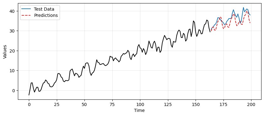
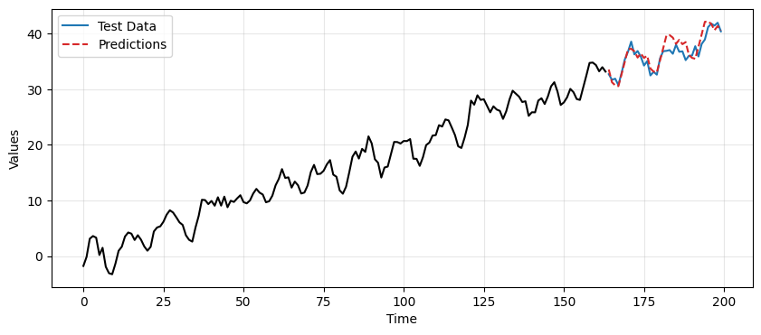
To obtain the final predictions we must first revert the seasonal differencing and then the 1st-order differencing.
# Reintegrating the seasonal differencing
reintegrated_seasonal = np.zeros(len(test_data_ar))
reintegrated_seasonal[:12] = diff_ar[-12:] + diff_preds[:12]
for i in range(12, len(test_data_ar)):
    reintegrated_seasonal[i] = reintegrated_seasonal[i-12] + diff_preds[i]

# Reintegrating 1st order differencing
reintegrated = reintegrated_seasonal.cumsum() + train_data_ar[-1]

_, ax = plt.subplots(1, 1, figsize=(10, 4))
run_sequence_plot(time[:len(train_data_ar)], train_data_ar, "", ax=ax)
ax.plot(time[len(train_data_ar):], test_data_ar, label='Test Data', color='tab:blue')
ax.plot(time[len(train_data_ar):], reintegrated, label='Predictions', linestyle='--', color='tab:red')
plt.legend();
Caution
It’s very easy to make errors with indices when reverting the differencing operations.
Also, the previous operations assume that there are no gaps between train and test data.
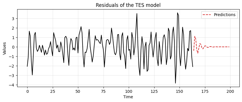
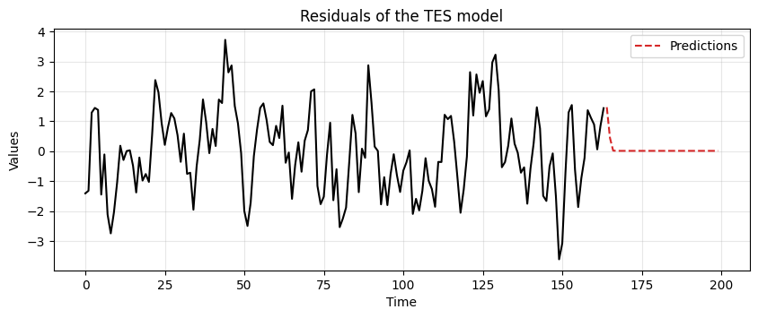
Predictions with TES-based approach#
Next, we consider the stationary data obtained by subtracting the trend and seasonality estimated with TES.
This time we use
tes_residto fit the AR(2) model and make forecasts.
model = ARIMA(tes_resid, order=(2,0,0))
model_fit = model.fit()

resid_preds = model_fit.forecast(steps=len(test_data_ar))

ax = run_sequence_plot(time[:len(train_data_ar)], tes_resid, "")
ax.plot(time[len(train_data_ar):], resid_preds, label='Predictions', linestyle='--', color='tab:red')
plt.title('Residuals of the TES model')
plt.legend();
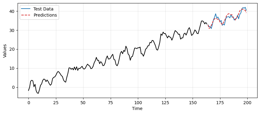
Then, we add back the trend and the seasonality to the predictions.
To do that, we first generate predictions for trend and seasonal components using TES.
Finally, we sum all the predictions to obtain the final result.
# Add back trend and seasonality to the predictions
tes_pred = tes.forecast(len(test_data_ar))
final_preds = tes_pred + resid_preds

_, ax = plt.subplots(1, 1, figsize=(10, 4))
run_sequence_plot(time[:len(train_data_ar)], train_data_ar, "", ax=ax)
ax.plot(time[len(train_data_ar):], test_data_ar, label='Test Data', color='tab:blue')
ax.plot(time[len(train_data_ar):], final_preds, label='Predictions', linestyle='--', color='tab:red')
plt.legend();
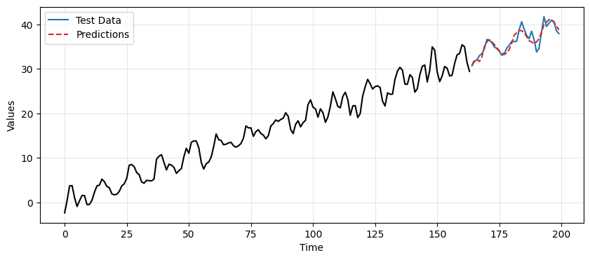
In this case we obtain better predictions using the TES-based approach compared to differencing.
We can quantify the difference in performance by computing the MSE.
mse_differencing = mean_squared_error(test_data_ar, reintegrated)
mse_tes = mean_squared_error(test_data_ar, final_preds)

print(f"MSE of differencing: {mse_differencing:.2f}")
print(f"MSE of TES: {mse_tes:.2f}")
MSE of differencing: 7.16
MSE of TES: 1.11
Moving Average (MA) models#
Another approach to modeling univariate time series is the moving average (MA) model.
The MA model is a linear regression of the current value of the series against the white noise of one or more of the previous values of the series.
The noise at each point is assumed to come from a normal distribution with mean 0 and constant variance.
The MA model is defined as:
where:
\(X(t)\): Time series value at time \(t\).
\(\mu\): Mean of the series.
\(\theta_1, \theta_2, \dots, \theta_q\): Coefficients of the model.
\(q\): Order of the MA model (number of lagged error terms).
\(\epsilon_t\): Error term (white noise) at time \(t\).
MA models capture the dependency between an observation and a residual error through a moving average applied to lagged observations.
Fitting MA estimates is more complicated than AR models because the error terms are not observable.
Therefore, iterative nonlinear fitting procedures need to be used.
MA models are less interpretable than AR models.
As AR models, also MA models require data to be stationary.
Attention
We talked about smoothing with moving averages in Lesson 3.
MA models are not the same as those smoothing techniques.
Each serves a different, important function.
We should not confuse the two.
MA model identification#
Before, for the AR model identification, we selected \(p\) as the lag after which the spikes in the PACF become nonsignificant.
To identify the order \(q\) of the MA model we do the same but we use the ACF plot instead.
Let’s see it through an example.
We generate some data from an MA(2) process with coefficients
[1.0, 0.7, 0.8].Again, the
1.0at the beginning refers to the zero-lag.
ma = np.array([1.0, 0.7, 0.8])  # MA parameters
ma_data = arma_generate_sample(np.array([1]), ma, nsample=len(time),
                               scale=1, burnin=1000) # MA process
_, ax = plt.subplots(1, 1, figsize=(5, 3))
plot_acf(ma_data, ax=ax, title="ACF of the MA process")
plt.tight_layout();
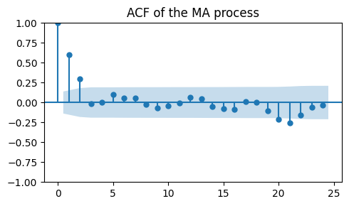
As expected, there is a cutoff after the second lag.
This indicates that the order of the MA model is \(q=2\).
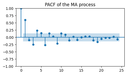
Characteristic of an MA process are the slowly decaying, alternative spikes in the PACF plot.
Note how this is complementary to what we saw for the AR process.
_, ax = plt.subplots(1, 1, figsize=(5, 3))
plot_pacf(ma_data, ax=ax, title="PACF of the MA process")
plt.tight_layout();
⚙ Try it yourself
Try modifying/adding/removing values in the
macoefficients inarma_generate_sample.Then, see how the ACF plot changes.
Example: forecasting with MA model#
We repeat the same procedure as in the AR example with a MA model.
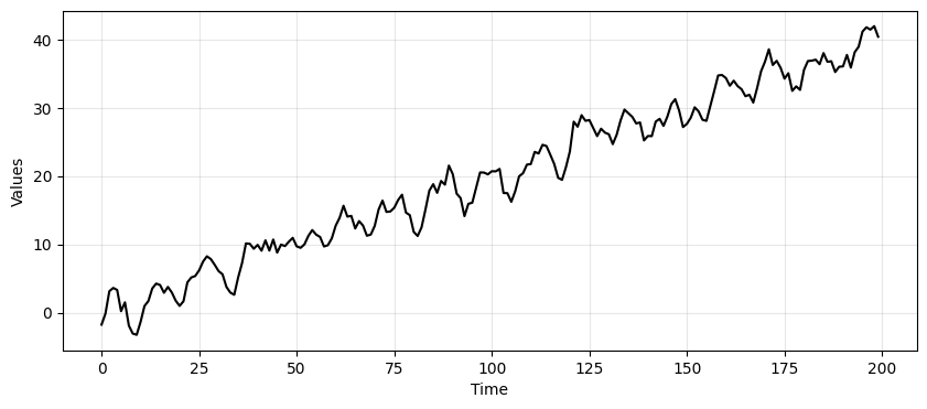
The only difference is that now we construct a time series using a MA process rather than an AR one.
time_series_ma = trend + seasonality + ma_data

_, ax = plt.subplots(1, 1, figsize=(10, 4))
run_sequence_plot(time, time_series_ma, "", ax=ax);
# Train/test split
train_data_ma = time_series_ma[:164]
test_data_ma = time_series_ma[164:]
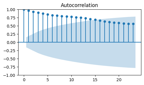
To identify the order \(q\) of the MA model we must look at the ACF plot.
Let’s start by computing the ACF of
train_data_ma, which looks very different from the ACF plot we obtained before for the MA process.
_, ax = plt.subplots(1, 1, figsize=(5, 3))
plot_acf(train_data_ma, ax=ax)
plt.tight_layout();
Also in this case, we need to make the time series stationary to obtain a meaningful ACF plot.
Like in the AR case, stationarity is needed to correctly estimate the MA coefficients.
Stationairty through differencing#
Like we did in the AR example, we will try to obtain stationaity through differencing.
diff_ma = train_data_ma[1:] - train_data_ma[:-1]
To verify that our data are stationary, we compute the ADF test before and after differentiation.
_, pvalue_ts, _, _, _, _ = adfuller(train_data_ma)
_, pvalue_diff, _, _, _, _ = adfuller(diff_ma)
print(f"p-value (original ts): {pvalue_ts:.3f}")
print(f"p-value (differenced ts): {pvalue_diff:.3f}")
p-value (original ts): 0.925
p-value (differenced ts): 0.000
We also plot the differenced data and compute the ACF.
_, axes = plt.subplots(1,2, figsize=(10, 3))
run_sequence_plot(time[1:len(train_data_ma)], diff_ma, "Differenced MA time series", ax=axes[0])
plot_acf(diff_ma, ax=axes[1])
plt.tight_layout();
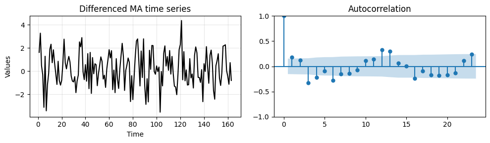
Like in the previous case, we have significant correlations at higher lags due to the seasonal component.
For comparison, we compute the ACF of:
the original MA process,
the time series after 1st order differencing,
the time series with both 1st order + seasonal differening.
diff_diff_ma = diff_ma[12:] - diff_ma[:-12]

_, axes = plt.subplots(1,3, figsize=(12, 3))
plot_acf(ma_data[:len(train_data_ma)], ax=axes[0], title="Original MA process")
plot_acf(diff_ma, ax=axes[1], title="1st order diff")
plot_acf(diff_diff_ma, ax=axes[2], title="1st order + seasonal diff")
plt.tight_layout();
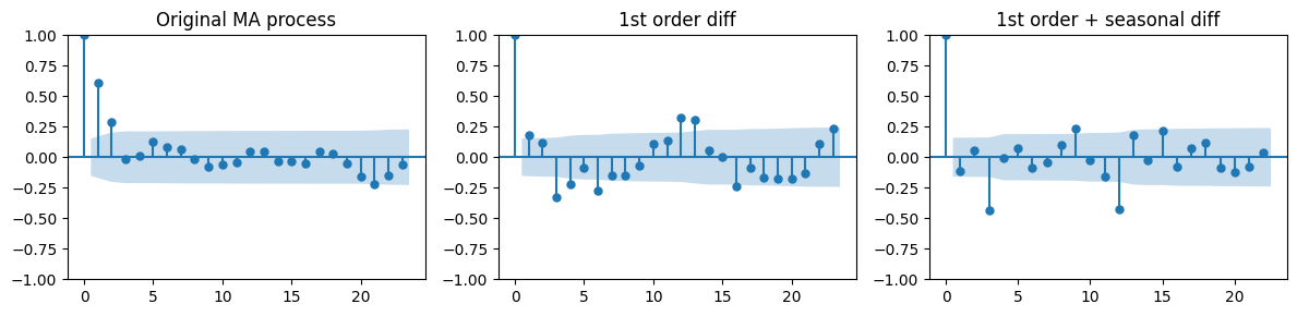
When taking both differencing the ACF plot looks very different.
The positive correlations at lags 1 and 2 are gone and a the first non-zero correlation appears at lag 3.
Like we saw in the AR case, this hints at an overdifferencing.
In conclusion, is not obvious which MA model to use from the analysis of the ACF plots.
The ACF after 1st order differencing suggests using order \(q=1\) or \(q=2\).
The ACF obtained after seasonal differencing suggests order \(q=3\), but we suspect overdifferencing.
Stationarity by subtracting estimated trend and seasonality#
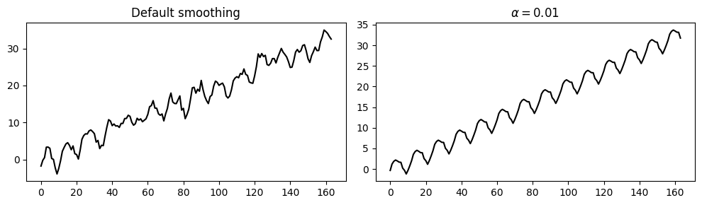
In the following we repeat the same procedure to estimate trend and seasonality with TES.
Since the MA process is more “noisy” that the AR process, we increase the level of smoothing by setting \(\alpha=0.01\).
As shown in the plot below, this leads to a smoother estimate of the trend and seasonality.
period, _, _ =fft_analysis(time_series_ma)
period = np.round(period).astype(int)

tes_ma_default = ExponentialSmoothing(train_data_ma, trend='add',
                           seasonal='add', seasonal_periods=period).fit(smoothing_level=None)
tes_ma = ExponentialSmoothing(train_data_ma, trend='add',
                           seasonal='add', seasonal_periods=period).fit(smoothing_level=0.01)
trend_and_seasonality_default = tes_ma_default.fittedvalues
trend_and_seasonality = tes_ma.fittedvalues

_, axes = plt.subplots(1, 2, figsize=(10, 3))
axes[0].plot(trend_and_seasonality_default, 'k')
axes[0].set_title('Default smoothing')
axes[1].plot(trend_and_seasonality, 'k')
axes[1].set_title('$\\alpha=0.01$')
plt.tight_layout();
Next, we compute the residuals by subtracting the estimated trend and seasonality.
Differently from the AR case, the ACF plots of the original MA process and the TES residuals are not so similar.
tes_resid_ma = train_data_ma - trend_and_seasonality

_, axes = plt.subplots(1, 2, figsize=(10, 3))
plot_acf(ma_data[:len(train_data_ma)], ax=axes[0], title="ACF Original MA process")
plot_acf(tes_resid, ax=axes[1], title="ACF of TES residuals")
plt.tight_layout();
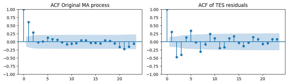
The ACF plot shows a significant spike at lag 3.
This suggests using a MA model with order \(q=3\) (even if data were generated with MA(2)).
As in the AR case, we compute predictions using both the differencing and the TES-based approach.
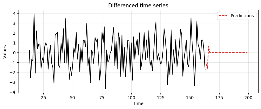
Predictions through differencing approach#
We start by fitting an MA model to
diff_diff_madata and compute the predictions.Note that, even if we generated the data with an MA(2) process, we use an MA(3) process since the ACF
diff_diff_mahad a large spike at lag 3.
# Fit the model
model = ARIMA(diff_diff_ma, order=(0,0,3))
model_fit = model.fit()

# Compute predictions
diff_preds = model_fit.forecast(steps=len(test_data_ma))

ax = run_sequence_plot(time[13:len(train_data_ma)], diff_diff_ma, "")
ax.plot(time[len(train_data_ma):], diff_preds, label='Predictions', linestyle='--', color='tab:red')
plt.title('Differenced time series')
plt.legend();
Then, we revert the two differencing operations to obtain the final predictions.
# Reintegrating the seasonal differencing
reintegrated_seasonal = np.zeros(len(test_data_ma))
reintegrated_seasonal[:12] = diff_ma[-12:] + diff_preds[:12]
for i in range(12, len(test_data_ma)):
    reintegrated_seasonal[i] = reintegrated_seasonal[i-12] + diff_preds[i]

# Reintegrating 1st order differencing
reintegrated = reintegrated_seasonal.cumsum() + train_data_ma[-1]

_, ax = plt.subplots(1, 1, figsize=(10, 4))
run_sequence_plot(time[:len(train_data_ma)], train_data_ma, "", ax=ax)
ax.plot(time[len(train_data_ma):], test_data_ma, label='Test Data', color='tab:blue')
ax.plot(time[len(train_data_ma):], reintegrated, label='Predictions', linestyle='--', color='tab:red')
plt.legend();
Predictions with TES-based approach#
This time we fit the MA model with
tes_resid_madata and compute the predictions.Notice that again we use an MA(3) model, even though we know the data was generated from an MA(2) process.
model = ARIMA(tes_resid_ma, order=(0,0,3))
model_fit = model.fit() # Fit the model

resid_preds = model_fit.forecast(steps=len(test_data_ma)) # Compute predictions

ax = run_sequence_plot(time[:len(train_data_ma)], tes_resid_ma, "")
ax.plot(time[len(train_data_ma):], resid_preds, label='Predictions', linestyle='--', color='tab:red')
plt.title('Residuals of the TES model')
plt.legend();
The final predictions are obtained by combining:
the predictions of the residuals from the MA model,
the prediction of the trend and seasonality from the TES model.
# Add back trend and seasonality to the predictions
tes_pred = tes_ma.forecast(len(test_data_ma))
final_preds = tes_pred + resid_preds

_, ax = plt.subplots(1, 1, figsize=(10, 4))
run_sequence_plot(time[:len(train_data_ma)], train_data_ma, "", ax=ax)
ax.plot(time[len(train_data_ma):], test_data_ma, label='Test Data', color='tab:blue')
ax.plot(time[len(train_data_ma):], final_preds, label='Predictions', linestyle='--', color='tab:red')
plt.legend();
This time the differencing approach gives better results but still worse than the TES-based approach.
mse_differencing = mean_squared_error(test_data_ma, reintegrated)
mse_tes = mean_squared_error(test_data_ma, final_preds)

print(f"MSE of differencing: {mse_differencing:.2f}")
print(f"MSE of TES: {mse_tes:.2f}")
MSE of differencing: 2.09
MSE of TES: 1.44
Summary#
AR vs MA Models#
AR Models |
MA Models |
|---|---|
Depend on past values of the series. |
Depend on past forecast errors. |
Suitable when past values have a direct influence on future values and for slowly changing time series |
Useful when the series is better explained by shocks or random disturbances, i.e., time series with sudden changes |
If the PACF drops sharply at a given lag \(p\), then use an AR model with order \(p\) |
If the ACF drops sharply at a given lag \(q\), then use an MA model with order \(q\) |
In this lecture we learned the basics of:
The Autocorrelation Function (ACF).
The Partial Autocorrelation Function (PACF).
Autoregressive (AR) models.
Choosing order \(p\).
Moving Average (MA) models.
Choosing order \(q\).
Combining smoothers to predict trend and seasonality with AR/MA models to predict the residuals.
Exercises#
Load the two time series
arma_ts1andarma_ts2by running the code below.
# Load the first time series
response = requests.get("https://zenodo.org/records/10951538/files/arma_ts3.npz?download=1")
response.raise_for_status()
arma_ts1 = np.load(BytesIO(response.content))['signal']
print(len(arma_ts1))

# Load the second time series
response = requests.get("https://zenodo.org/records/10951538/files/arma_ts4.npz?download=1")
response.raise_for_status()
arma_ts2 = np.load(BytesIO(response.content))['signal']
print(len(arma_ts2))
479
1000
For each time series:
Split the time series in train and test.
Use the last 30 values as test for the first time series.
Use the last 100 as test for the second time series.
Make the time series stationary.
Determine the order \(p\) of an AR model.
Compute the prediction of the test data with the AR(\(p\)) model.
Determine the order \(q\) of a MA model.
Compute the prediction of the test data with the MA(\(q\)) model.