ARMA, ARIMA, SARIMA#

Overview#
In the previous chapters, we covered stationarity, smoothing, trend, seasonality, and autocorrelation, and built two different models:
MA models: The current value of the series depends linearly on the series’ mean and a set of prior (observed) white noise error terms.
AR models: The current value of the series depends linearly on its own previous values and on a stochastic term (an imperfectly predictable term).
In this chapter we will review these concepts and combine the AR and MA models into three more complicated ones.
In particular, we will cover:
Autoregressive Moving Average (ARMA) models.
Autoregressive Integrated Moving Average (ARIMA) models.
SARIMA models (ARIMA model for data with seasonality).
Selecting the best model.
ARMA#
The ARMA model (also known as the Box-Jenkins approach) combines two models:
An autoregressive (AR) model of order \(p\).
A moving average (MA) model of order \(q\).
When we have autocorrelation between outcomes and their ancestors, there will be a pattern in the time series.
This relationship can be modeled using an ARMA model.
It allows us to predict the future with a confidence level proportional to the strength of the relationship and the proximity to known values (prediction weakens the further out we go).
Note
ARMA models assume the time series is stationary.
A good rule of thumb is to have at least 100 observations when fitting an ARMA model.
Example data#
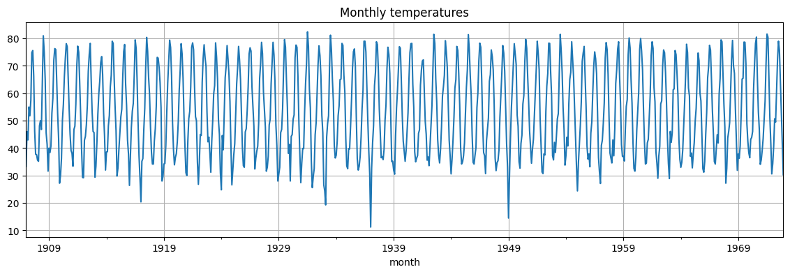
In the following, we’ll look at the monthly average temperatures between 1907-1972.
# load data and convert to datetime
monthly_temp = pd.read_csv('https://zenodo.org/records/10951538/files/arima_temp.csv?download=1',
                           skipfooter=2,
                           header=0,
                           index_col=0,
                           names=['month', 'temp'],
                           engine='python')
monthly_temp.index = pd.to_datetime(monthly_temp.index)
This is how the data looks like.
monthly_temp.head()
| temp | |
|---|---|
| month | |
| 1907-01-01 | 33.3 |
| 1907-02-01 | 46.0 |
| 1907-03-01 | 43.0 |
| 1907-04-01 | 55.0 |
| 1907-05-01 | 51.8 |
These are some statistics.
monthly_temp.describe()
| temp | |
|---|---|
| count | 792.000000 |
| mean | 53.553662 |
| std | 15.815452 |
| min | 11.200000 |
| 25% | 39.675000 |
| 50% | 52.150000 |
| 75% | 67.200000 |
| max | 82.400000 |
This is the run sequence plot.
monthly_temp['temp'].plot(grid=True, figsize=(14, 4), title="Monthly temperatures");
We compute the annual mean and plot it on top of the data.
# Compute annual mean
annual_temp = monthly_temp.resample('YE').mean()
annual_temp.index.name = 'year'

plt.figure(figsize=(14, 4))
plt.plot(monthly_temp, label="Monthly Temperatures")
plt.plot(annual_temp, label="Annual Mean")
plt.grid(); plt.legend();
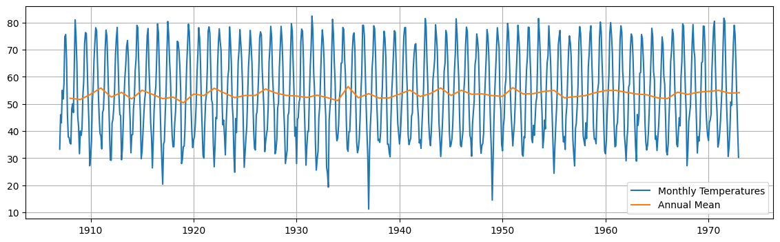
This gives us an indication that the mean is rather constant over the years.
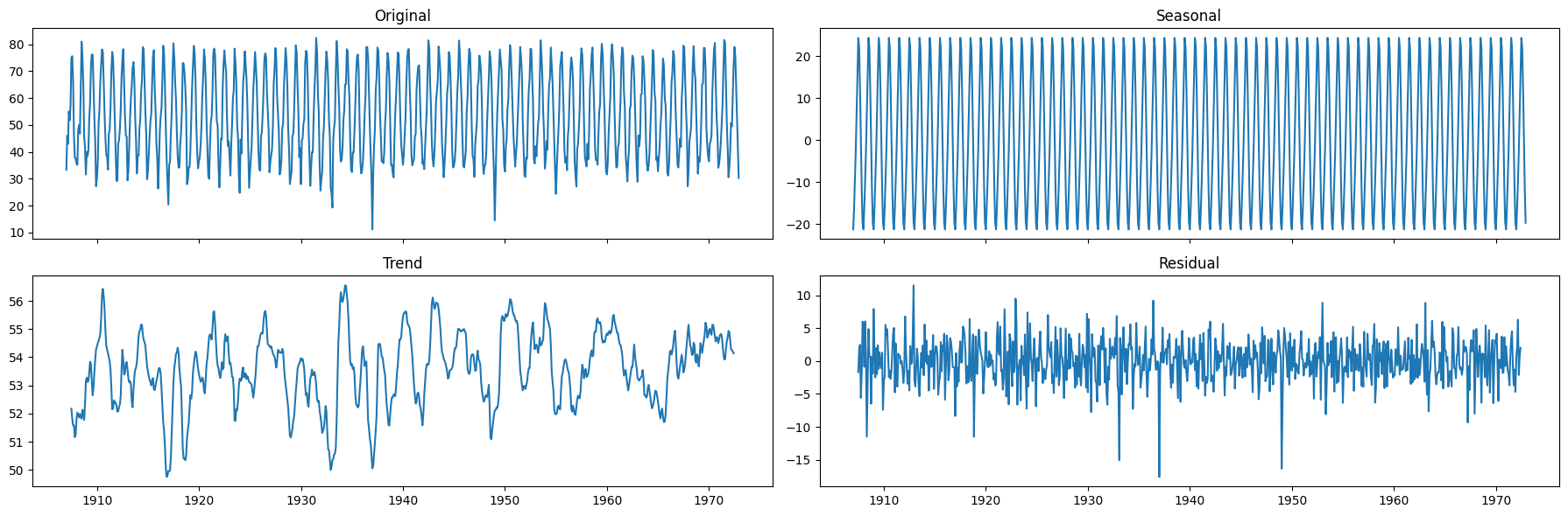
We can extract further information abouth the underlying trend and seasonality by performing a seasonal decomposition.
We can use both the
seasonal_decomposeand theSTLmethods.
decomposition = seasonal_decompose(x=monthly_temp['temp'], model='additive', period=12)
seasonal, trend, resid = decomposition.seasonal, decomposition.trend, decomposition.resid

fig, axs = plt.subplots(2,2, sharex=True, figsize=(18,6))
axs[0,0].plot(monthly_temp['temp'])
axs[0,0].set_title('Original')
axs[0,1].plot(seasonal)
axs[0,1].set_title('Seasonal')
axs[1,0].plot(trend)
axs[1,0].set_title('Trend')
axs[1,1].plot(resid)
axs[1,1].set_title('Residual')
plt.tight_layout()
decomposition = STL(endog=monthly_temp['temp'], period=12, seasonal=13, robust=True).fit()
seasonal, trend, resid = decomposition.seasonal, decomposition.trend, decomposition.resid

fig, axs = plt.subplots(2,2, sharex=True, figsize=(18,6))
axs[0,0].plot(monthly_temp['temp'])
axs[0,0].set_title('Original')
axs[0,1].plot(seasonal)
axs[0,1].set_title('Seasonal')
axs[1,0].plot(trend)
axs[1,0].set_title('Trend')
axs[1,1].plot(resid)
axs[1,1].set_title('Residual')
plt.tight_layout()
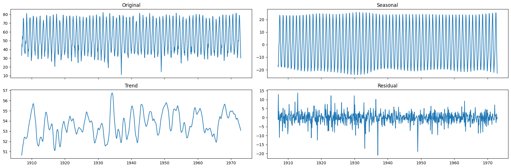
The seasonality is well defined.
There doesn’t seem to be a strong, time-varying trend in the data.
We can assume the trend is almost constant.
ARMA modeling stages#
There are three stages in building an ARMA model:
Model identification.
Model estimation.
Model evaluation.
Model identification#
Model identification consists in finding the orders \(p\) and \(q\) of AR and MA components.
Before performing model identification we need to:
Determine if the time series is stationary.
Determine if the time series has seasonal component.
Determine stationarity#
We will use tools we already know (ADF test).
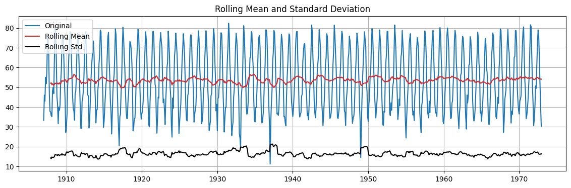
We can also look at the rolling mean and std.
Attention
Before we continue, let’s consider the result below.
sinusoid = np.sin(np.arange(200))
_, pvalue, _, _, _, _ = adfuller(sinusoid)
print(f'p-value: {pvalue}')
p-value: 0.0
Periodic signals, by their nature, have means and variances that repeat over the period of the cycle.
This implies that their statistical properties are functions of time within each period.
For instance, the mean of a periodic signal over one cycle may be constant.
However, when considering any point in time relative to the cycle, the instantaneous mean of the signal can vary.
Similarly, the variance can fluctuate within the cycle.
The ADF test specifically looks for a unit root (more on this later on).
A unit root indicates that shocks to the time series have a permanent effect, causing drifts in the level of the series.
A sinusoidal function, by contrast, is inherently mean-reverting within its cycles.
After a peak a sinusoid reverts to its mean and any “shock” in terms of phase shift or amplitude change does not alter its oscillatory nature.
It’s crucial to note that the ADF test’s conclusion of stationarity for a sinusoid does not imply that the sinusoid is stationary.
The test’s conclusion is about the absence of a unit root.
This does not imply that the mean and variance are constant within the periodic fluctuations.
def adftest(series, plots=True):
    out = adfuller(series, autolag='AIC')
    print(f'ADF Statistic: {out[0]:.2f}')
    print(f'p-value: {out[1]:.3f}')
    print(f"Critical Values: {[f'{k}: {r:.2f}' for r,k in zip(out[4].values(), out[4].keys())]}\n")

    if plots:
        # Compute rolling statistics
        rolmean = series.rolling(window=12).mean()
        rolstd = series.rolling(window=12).std()

        # Plot rolling statistics:
        plt.figure(figsize=(14, 4))
        plt.plot(series, color='tab:blue',label='Original')
        plt.plot(rolmean, color='tab:red', label='Rolling Mean')
        plt.plot(rolstd, color='black', label = 'Rolling Std')
        plt.legend(loc='best')
        plt.title('Rolling Mean and Standard Deviation')
        plt.grid();
# run ADF on monthly temperatures
adftest(monthly_temp.temp)
ADF Statistic: -6.48
p-value: 0.000
Critical Values: ['1%: -3.44', '5%: -2.87', '10%: -2.57']
# run ADF on annual means
adftest(annual_temp.temp, plots=False)
ADF Statistic: -7.88
p-value: 0.000
Critical Values: ['1%: -3.54', '5%: -2.91', '10%: -2.59']
The \(p\)-value indicates that the time series is stationary…
… even if it clearly has a periodic component.
The rolling mean and rolling standard deviation seem globally constant along the time series…
… even if they change locally within the period.
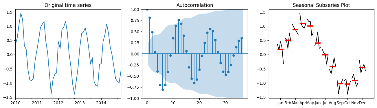
Determine seasonality#
We can determine if seasonality is present by using the following tools:
Autocorrelation plot.
Seasonal subseries plot (month plot).
Fourier Transform.
Let’s first look how these plots look like on synthetic data
# Generate synthetic time series data
dates = pd.date_range(start='2010-01-01', periods=60, freq='ME')  # Monthly data for 5 years
seas = 12 # change this and see how the plots change
data = (np.sin(np.arange(60)*2*np.pi/seas) +
        np.random.normal(loc=0, scale=0.2, size=60))  # Seasonal data with noise
series = pd.Series(data, index=dates)
fig, axes = plt.subplots(1,3,figsize=(16,4))
series.plot(ax=axes[0], title="Original time series")

# ACF Plot
plot_acf(series, lags=36, ax=axes[1]);

# Convert series to a DataFrame and add a column for the month
df = series.to_frame(name='Value')
df['Month'] = df.index.month

# Seasonal Subseries Plot
month_plot(df['Value'], ax=axes[2]); axes[2].set_title("Seasonal Subseries Plot");
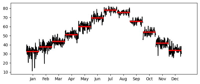
Let’s look at the real data now.
_, ax = plt.subplots(1,1, figsize=(7,3))
month_plot(monthly_temp, ax=ax)
plt.tight_layout();
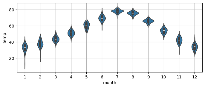
Notice that a
violinplotcan give a very similar information to themonth_plot.
_, ax = plt.subplots(1,1, figsize=(8,3))
sns.violinplot(x=monthly_temp.index.month,
               y=monthly_temp.temp, ax=ax) # notice the indexing on the x by month
plt.grid();
Finally, to obtain the numerical value of the main periodicity we can use the Foruier Transfrom.
Here, we’ll use the function we defined in the first lecture.
dominant_period, _, _ = fft_analysis(monthly_temp['temp'].values)
print(f"Dominant period: {np.round(dominant_period)}")
Dominant period: 12.0
Remove the main seasonality#
In this case, it is clear that the main seasonality is \(L=12\).
We can remove it with a seasonal differencing.
monthly_temp['Seasonally_Differenced'] = monthly_temp['temp'].diff(12)
# Drop nan
monthly_temp_clean = monthly_temp.dropna()
monthly_temp_clean
| temp | Seasonally_Differenced | |
|---|---|---|
| month | ||
| 1908-01-01 | 35.6 | 2.3 |
| 1908-02-01 | 35.2 | -10.8 |
| 1908-03-01 | 48.1 | 5.1 |
| 1908-04-01 | 50.0 | -5.0 |
| 1908-05-01 | 46.8 | -5.0 |
| ... | ... | ... |
| 1972-08-01 | 75.6 | -4.9 |
| 1972-09-01 | 64.1 | -1.7 |
| 1972-10-01 | 51.7 | 0.6 |
| 1972-11-01 | 40.3 | -1.5 |
| 1972-12-01 | 30.3 | -0.3 |
780 rows × 2 columns
⚙ Try it yourself
Try redoing the previous plots on the differenced data!
Identifying \(p\) and \(q\)#
As we learned in the previous chapter, we will identify the AR order \(p\) and the MA order \(q\) with:
Autocorrelation function (ACF) plot.
Partial autocorrelation function (PACF) plot.
AR(\(p\))
The order of the AR model is identified as follows:
Plot 95% confidence interval on the PACF (done as default by statsmodels).
Choose lag \(p\) such that the partial autocorrelation becomes insignificant for \(p+1\) and beyond.
If a process depends on previous values of itself then it is an AR process.
If it depends on previous errors than it is an MA process.
An AR process propagates shocks infinitely.
AR processes will exhibit exponential decay in ACF and a cut-off in PACF.
_, ax = plt.subplots(1, 1, figsize=(5, 3))
plot_pacf(monthly_temp_clean['Seasonally_Differenced'], lags=20, ax=ax);
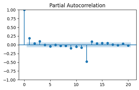
It looks like the PACF becomes zero at lag 2.
However there is a non-zero partial autocorrelation at lag 3.
The optimal value might be \(p=1\), \(p=2\), or \(p=3\).
Note that there are high partial autocorrelations at higher lags, especially 12.
This is an effect from seasonality and seasonal differencing.
It should not be accounted for when choosing \(p\).
MA(\(q\))
The order of the MA model is identified as follows:
Plot 95% confidence interval on the ACF (default in statsmodels).
Choose lag \(q\) such that ACF becomes statistically zero for \(q+1\) and beyond.
MA models do not propagate shocks infinitely; they die after \(q\) lags.
MA processes will exhibit exponential decay in PACF and a cut-off in ACF.
_, ax = plt.subplots(1, 1, figsize=(5, 3))
plot_acf(monthly_temp_clean['Seasonally_Differenced'], lags=20, ax=ax);
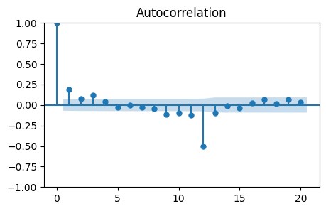
Also in this case there are non-zero autocorrelations at lags 1 and 3.
So, the values to try are \(q=1\), \(q=2\), or \(q=3\).
Model estimation#
Once the orders \(p\) and \(q\) are identified is necessary to estimate parameters \(\phi_1, \dots, \phi_p\) of the AR part and parameters \(\theta_1, \dots, \theta_q\) of the MA part.
Estimating the parameters of an ARMA model is a complicated, nonlinear problem.
Nonlinear least squares and maximum likelihood estimation are common approaches.
Software packages will fit the ARMA model for us.
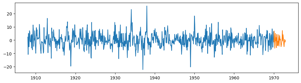
We split the data in two parts:
the training set, that will be used to fit the model’s parameters.
the test set, that will be used later on to evaluate the prediction performance of the model on unseen data.
train = monthly_temp_clean['Seasonally_Differenced'][:-36]
test = monthly_temp_clean['Seasonally_Differenced'][-36:]

plt.figure(figsize=(12,3))
plt.plot(train)
plt.plot(test);
model = ARIMA(train, order=(3, 0, 3))  # ARIMA with d=0 is equivalent to ARMA
fit_model = model.fit()

print(fit_model.summary())
                                 SARIMAX Results
==================================================================================
Dep. Variable:     Seasonally_Differenced   No. Observations:                  744
Model:                     ARIMA(3, 0, 3)   Log Likelihood               -2248.077
Date:                    Fri, 01 May 2026   AIC                           4512.155
Time:                            09:22:53   BIC                           4549.051
Sample:                        01-01-1908   HQIC                          4526.377
                             - 12-01-1969
Covariance Type:                      opg
==============================================================================
                 coef    std err          z      P>|z|      [0.025      0.975]
------------------------------------------------------------------------------
const          0.0652      0.243      0.268      0.789      -0.412       0.542
ar.L1         -0.0926      0.141     -0.658      0.511      -0.369       0.183
ar.L2         -0.8298      0.023    -35.651      0.000      -0.875      -0.784
ar.L3          0.0460      0.123      0.375      0.708      -0.194       0.286
ma.L1          0.2831      0.139      2.030      0.042       0.010       0.556
ma.L2          0.9967      0.012     85.460      0.000       0.974       1.020
ma.L3          0.2395      0.140      1.714      0.087      -0.034       0.513
sigma2        24.3084      1.007     24.140      0.000      22.335      26.282
===================================================================================
Ljung-Box (L1) (Q):                   0.00   Jarque-Bera (JB):                57.00
Prob(Q):                              0.97   Prob(JB):                         0.00
Heteroskedasticity (H):               0.77   Skew:                             0.12
Prob(H) (two-sided):                  0.04   Kurtosis:                         4.34
===================================================================================

Warnings:
[1] Covariance matrix calculated using the outer product of gradients (complex-step).
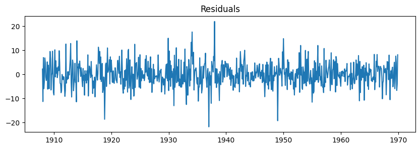
ARMA Model Validation#
How do we know if our ARMA model is good enough?
We can check the residuals, i.e., what the model was not able to fit.
The residuals should approximate a Gaussian distribution (aka white noise).
Otherwise, we might need to select a better model.
residuals = fit_model.resid

plt.figure(figsize=(10,3))
plt.plot(residuals)
plt.title("Residuals");
🤔 How to test if the residuals look like noise?
We will use both visual inspection and statistical tests.
Visual inspection:
ACF plot.
Histogram.
QQ plot.
Statistical tests:
Normality.
Autocorrelation.
Heteroskedasticity.
Visual inspection#
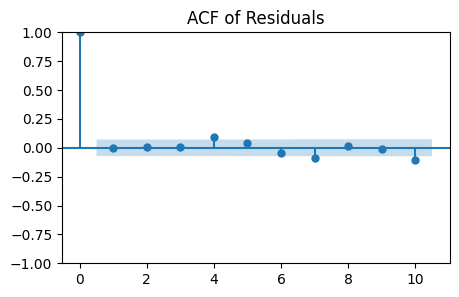
ACF plot
Checks for any autocorrelation in the residuals.
White noise should show no significant autocorrelation at all lags.
_, ax = plt.subplots(1, 1, figsize=(5, 3))
plot_acf(residuals, lags=10, ax=ax)
plt.title('ACF of Residuals');
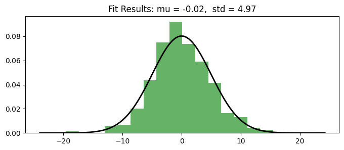
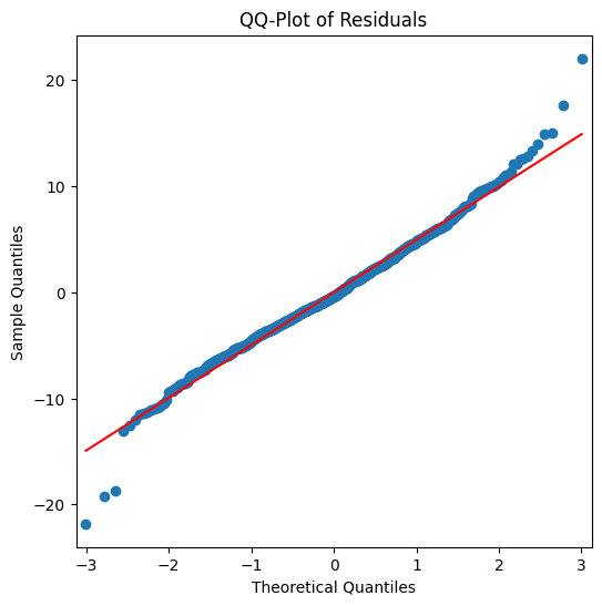
Histogram and QQ-Plot
Assess the normality of the residuals.
White noise should ideally follow a normal distribution.
plt.figure(figsize=(8,3))
plt.hist(residuals, bins=20, density=True, alpha=0.6, color='g') # Histogram
# Add the normal distribution curve
xmin, xmax = plt.xlim()
x = np.linspace(xmin, xmax, 100)
p = stats.norm.pdf(x, np.mean(residuals), np.std(residuals))
plt.plot(x, p, 'k', linewidth=2)
title = "Fit Results: mu = %.2f,  std = %.2f" % (np.mean(residuals), np.std(residuals))
plt.title(title);
# QQ-Plot
_, ax = plt.subplots(1, 1, figsize=(6, 6))
qqplot(residuals, line='s', ax=ax)
plt.title('QQ-Plot of Residuals');
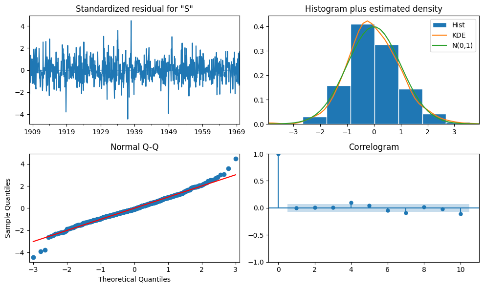
The plots are conveniently summarized in the function
plot_diagnostics()that can be called on the fit model.
fit_model.plot_diagnostics(figsize=(10, 6))
plt.tight_layout();
Statistical tests#
Normality: Jarque-Bera and Shapiro-Wilk tests
\(H_0\): the residuals are normally distributed.
norm_val, norm_p, skew, kurtosis = fit_model.test_normality('jarquebera')[0]
print('Normality (Jarque-Bera) p-value:{:.3f}'.format(norm_p))
Normality (Jarque-Bera) p-value:0.000
shapiro_test = stats.shapiro(residuals)
print(f'Normality (Shapiro-Wilk) p-value: {shapiro_test.pvalue:.3f}')
Normality (Shapiro-Wilk) p-value: 0.000
The small \(p\)-values allow us to reject \(H_0\).
Conclusion: the residuals are not normally distributed.
Is this a contraddiction?
Note
For reference, let’s see what these tests say about data that are actually normally distributed.
Try executing the cell below multiple times and see how much the results changes each time.
These tests start to be reliable only for large sample sizes (\(N>5000\)).
# generate random normal data
normal_data = np.random.normal(loc=0, scale=1, size=1000)

jb_test = stats.jarque_bera(normal_data)
print(f'Normality (Jarque-Bera) p-value: {jb_test.pvalue:.3f}')

shapiro_test = stats.shapiro(normal_data)
print(f'Normality (Shapiro-Wilk) p-value: {shapiro_test.pvalue:.3f}')
Normality (Jarque-Bera) p-value: 0.811
Normality (Shapiro-Wilk) p-value: 0.938
Autocorrelation: Ljung-Box test
\(H_0\): the residuals are independently distributed (no autocorrelation).
There is a \(p\)-value for each lag.
Here we just take the mean, but one might also want to look at the at largest lag (
pval[-1]).It is also not always obvious to select how many lags should be used in the test…
statistic, pval = fit_model.test_serial_correlation(method='ljungbox', lags=10)[0]
print(f'Ljung-Box p-value: {pval.mean():.3f}')
Ljung-Box p-value: 0.355
Autocorrelation: Durbin Watson test
Tests autocorrelation in the residuals.
We want something between 1-3.
2 is ideal (no serial correlation).
durbin_watson = ss.stats.stattools.durbin_watson(
    fit_model.filter_results.standardized_forecasts_error[0, fit_model.loglikelihood_burn:])
print('Durbin-Watson: d={:.2f}'.format(durbin_watson))
Durbin-Watson: d=2.00
Heteroskedasticity test
Tests for change in variance between residuals.
\(H_0\): no heteroskedasticity.
\(H_0\) indicates different things based on the alternative \(H_A\):
\(H_A\): Increasing, \(H_0\): the variance is not increasing throughout the series.
\(H_A\): Decreasing, \(H_0\): the variance is not decreasing throughout the series.
\(H_A\): Two-sided (default), \(H_0\): the variance does not increase nor decrease throughout the series.
_, pval = fit_model.test_heteroskedasticity('breakvar', alternative='increasing')[0]
print(f'H_a: Increasing - pvalue:{pval:.3f}')
H_a: Increasing - pvalue:0.980
_, pval = fit_model.test_heteroskedasticity('breakvar', alternative='decreasing')[0]
print(f'H_a: Decreasing - pvalue:{pval:.3f}')
H_a: Decreasing - pvalue:0.020
_, pval = fit_model.test_heteroskedasticity('breakvar', alternative='two-sided')[0]
print(f'H_a: Two-sided - pvalue:{pval:.3f}')
H_a: Two-sided - pvalue:0.039
Summary of our tests
Independence:
✅ ACF plot.
✅ Ljung-Box test.
✅ Durbin Watson test.
Normality:
✅ Histogram/Density plot.
🤔 QQ-plot
❌ Jarque-Bera (reliable for large sample size).
❌ Shapiro-Wilk (reliable for large sample size).
Heteroskedasticity
❌ Heteroskedasticity test.
The tests are a bit inconclusive.
There is no strong evidence that the model is either very good or very bad.
It is probably wise to try other candidate models, e.g.,
ARMA(2,0,2), and repeat the tests.
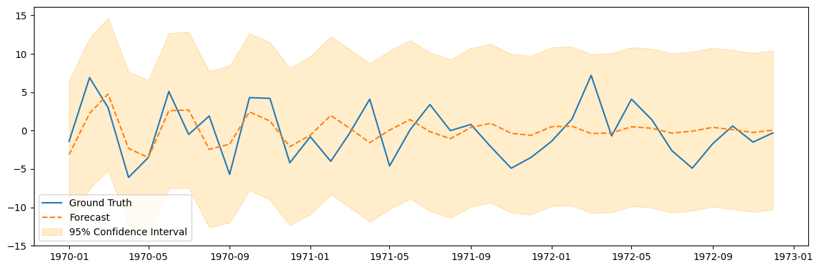
ARMA Model Predictions#
Once the model is fit, we can use it to predict the test data.
The predictions come in the form of a distribution.
In other words, ARMA performs a probabilistic forecasting.
The mean (mode) of this distribution correspond to the most likely value and correspond to our forecast.
The rest of the distribution can be used to compute confidence intervals.
pred_summary = fit_model.get_prediction(test.index[0], test.index[-1]).summary_frame()

plt.figure(figsize=(12, 4))
plt.plot(test.index, test, label='Ground Truth')
plt.plot(test.index, pred_summary['mean'], label='Forecast', linestyle='--')
plt.fill_between(test.index, pred_summary['mean_ci_lower'], pred_summary['mean_ci_upper'],
                 color='orange', alpha=0.2, label='95% Confidence Interval')
plt.legend()
plt.tight_layout();
ARIMA Model#
ARIMA stands for Auto Regressive Integrated Moving Average.
ARIMA models have three components:
AR model.
Integrated component (more on this shortly).
MA model.
The ARIMA model is denoted ARIMA(\(p, d, q\)).
\(p\) is the order of the AR model.
\(d\) is the number of times to difference the data.
\(q\) is the order of the MA model.
\(p\), \(d\), and \(q\) are nonnegative integers.
As we saw previously, differencing nonstationary time series data one or more times can make it stationary.
That’s the role of the integrated (I) component of ARIMA.
\(d\) is the number of times to perform a lag 1 difference on the data.
\(d=0\): no differencing.
\(d=1\): difference once.
\(d=2\): difference twice.
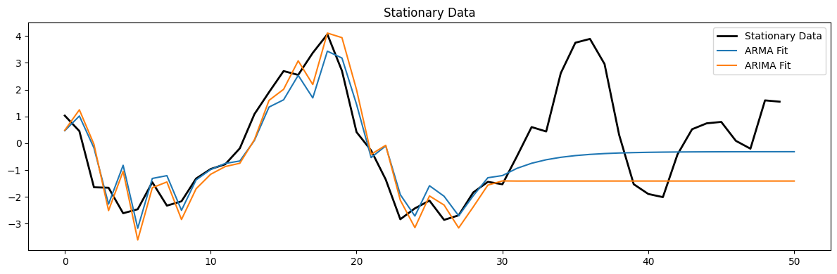
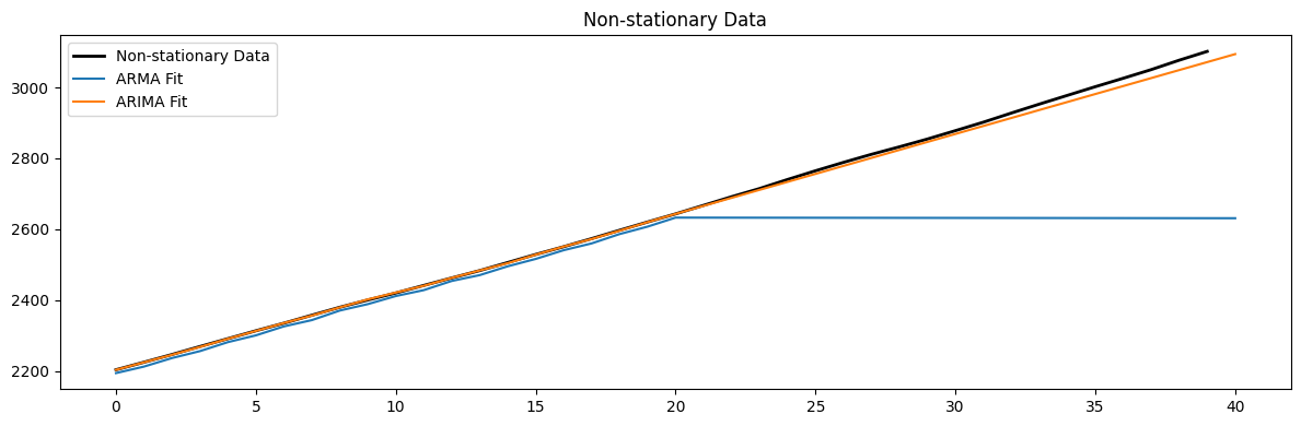
The ARMA model is suitable for stationary time series where the mean and variance do not change over time.
The ARIMA model effectively models non-stationary time series by differencing the data.
In practice, ARIMA makes the time series stationary before applying the ARMA model.
Let’s see it with an example.
# Generate synthetic stationary data with an ARMA(1,1) process
n = 250
ar_coeff = np.array([1, -0.7]) # The first value (lag 0) is always 1. AR coeff are negated.
ma_coeff = np.array([1, 0.7])  # The first value (lag 0) and is always 1
arma_data = ss.tsa.arima_process.ArmaProcess(ar_coeff, ma_coeff).generate_sample(
    nsample=n, burnin=1000)
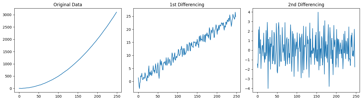
# Generate a synthetic non-stationary data (needs to be differenced twice to be stationary)
t = np.arange(n)
non_stationary_data = 0.05 * t**2 + arma_data  # Quadratic trend

fig, axes = plt.subplots(1, 3, figsize=(14, 4))
axes[0].plot(non_stationary_data)
axes[0].set_title('Original Data')
axes[1].plot(diff(non_stationary_data, k_diff=1))
axes[1].set_title('1st Differencing')
axes[2].plot(diff(non_stationary_data, k_diff=2))
axes[2].set_title('2nd Differencing')
plt.tight_layout();
# Fit models to stationary data
arma_model = ARIMA(arma_data[:-20], order=(1, 0, 1)).fit()
arima_model = ARIMA(arma_data[:-20], order=(1, 1, 1)).fit()

plt.figure(figsize=(12, 4))
plt.plot(arma_data[-50:], 'k', label='Stationary Data', linewidth=2)
plt.plot(arma_model.predict(200,250), label='ARMA Fit')
plt.plot(arima_model.predict(200, 250), label='ARIMA Fit')
plt.legend()
plt.title('Stationary Data')
plt.tight_layout();

print(len(arma_model.predict(10)))
220
# Fit models to non-stationary data
arma_model = ARIMA(non_stationary_data[:-20], order=(1, 0, 1)).fit()
arima_model = ARIMA(non_stationary_data[:-20], order=(1, 2, 1)).fit()

plt.figure(figsize=(12, 4))
plt.plot(non_stationary_data[-40:], 'k', label='Non-stationary Data', linewidth=2)
plt.plot(arma_model.predict(210,250), label='ARMA Fit')
plt.plot(arima_model.predict(210,250), label='ARIMA Fit')
plt.legend()
plt.title('Non-stationary Data')
plt.tight_layout();
SARIMA#
To apply ARMA and ARIMA, we must remove the seasonal component.
After computing the predictions we had to put the seasonal component back.
It would be convenient to directly work on data with seasonality.
SARIMA is an extension of ARIMA that includes seasonal terms.
The model is specified as SARIMA \((p, d, q) \times (P, D, Q, s)\):
Regular ARIMA components \((p, d, q)\).
Seasonal components \((P, D, Q, s)\) where:
\(P\): Seasonal autoregressive order.
\(D\): Seasonal differencing order.
\(Q\): Seasonal moving average order.
\(s\): Number of time steps for a single seasonal period.
How to select the values \(s, P, D, Q\)?
\(s\):
Is the main seasonality in the data.
We already know how to find it.
\(P\) and \(Q\):
A spike at \(s\)-th lag (and potentially multiples of \(s\)) should be present in the PACF/ACF plots.
For example, if \(s = 12\), there could be spikes at \((s*n)^{th}\) lags too.
Pick out the lags with largest spikes as candidates for \(P\) or \(Q\).
\(D\):
Is the number of seasonal differencing required to make the time series stationary.
Is often determined by trial and error or by examining the seasonally differenced data.
Tip
Before selecting \(P\) and \(Q\), ensure that the series is seasonally stationary by applying seasonal differencing if needed (\(D\)).
Look the ACF plot to identify the seasonal moving average order \(Q\).
Look for significant autocorrelations at seasonal lags (multiples of \(s\)).
If the ACF plot shows a sharp cut-off in the seasonal lags, it suggests the order of the seasonal MA component (\(Q\)).
Look at the PACF plot to identify the seasonal autoregressive order \(P\).
Look for significant spikes at multiples of the seasonality \(s\).
A sharp cut-off in the PACF at a seasonal lag suggests the order of the seasonal AR terms (\(P\)) needed.
diff_ts = monthly_temp['temp'].diff(periods=12).dropna()

fig = plt.figure(figsize=(10, 6))
ax1 = plt.subplot2grid((2, 2), (0, 0), colspan=2)
ax1.plot(diff_ts)
ax2 = plt.subplot2grid((2, 2), (1, 0))
plot_pacf(diff_ts, lags=80, ax=ax2)
ax3 = plt.subplot2grid((2, 2), (1, 1))
plot_acf(diff_ts, lags=80, ax=ax3)
plt.tight_layout();
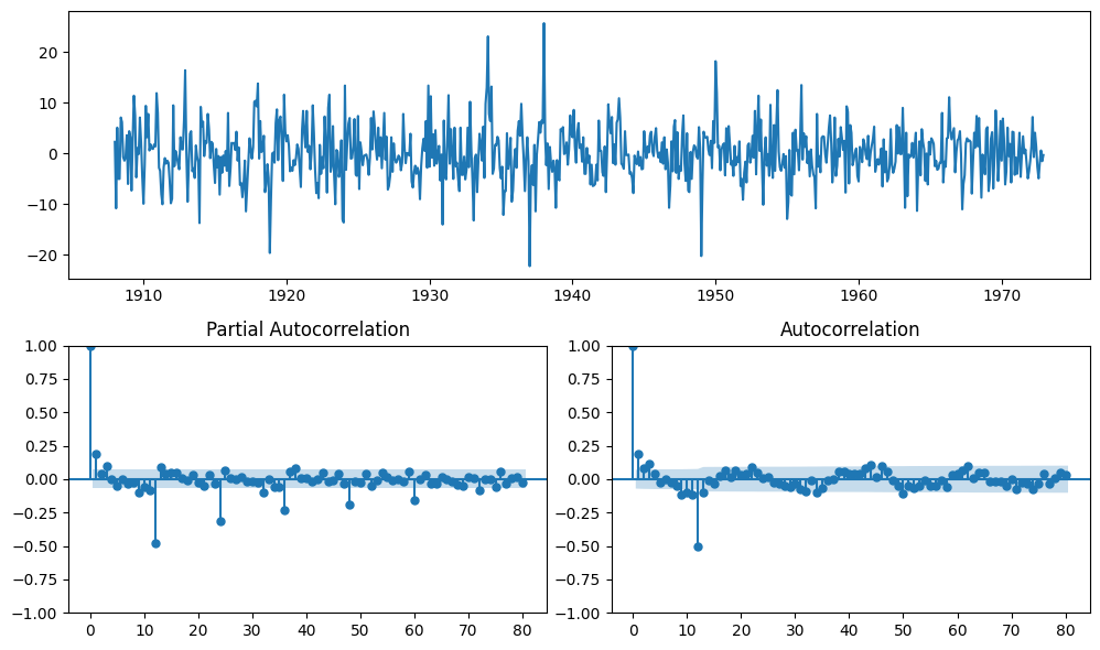
# fit SARIMA monthly based on helper plots
sar = ss.tsa.statespace.sarimax.SARIMAX(monthly_temp[:750].temp,
                                order=(2,1,2),
                                seasonal_order=(0,1,1,12),
                                trend='c').fit(disp=False)
sar.summary()
| Dep. Variable: | temp | No. Observations: | 750 |
|---|---|---|---|
| Model: | SARIMAX(2, 1, 2)x(0, 1, [1], 12) | Log Likelihood | -2026.037 |
| Date: | Fri, 01 May 2026 | AIC | 4066.074 |
| Time: | 09:23:00 | BIC | 4098.292 |
| Sample: | 01-01-1907 | HQIC | 4078.499 |
| - 06-01-1969 | |||
| Covariance Type: | opg |
| coef | std err | z | P>|z| | [0.025 | 0.975] | |
|---|---|---|---|---|---|---|
| intercept | -6.806e-05 | 0.000 | -0.380 | 0.704 | -0.000 | 0.000 |
| ar.L1 | -0.7665 | 0.242 | -3.166 | 0.002 | -1.241 | -0.292 |
| ar.L2 | 0.1795 | 0.050 | 3.575 | 0.000 | 0.081 | 0.278 |
| ma.L1 | -0.0502 | 0.255 | -0.197 | 0.844 | -0.550 | 0.450 |
| ma.L2 | -0.9478 | 0.244 | -3.878 | 0.000 | -1.427 | -0.469 |
| ma.S.L12 | -0.9826 | 0.041 | -23.780 | 0.000 | -1.064 | -0.902 |
| sigma2 | 13.3745 | 1.079 | 12.392 | 0.000 | 11.259 | 15.490 |
| Ljung-Box (L1) (Q): | 0.07 | Jarque-Bera (JB): | 204.11 |
|---|---|---|---|
| Prob(Q): | 0.79 | Prob(JB): | 0.00 |
| Heteroskedasticity (H): | 0.77 | Skew: | -0.55 |
| Prob(H) (two-sided): | 0.04 | Kurtosis: | 5.33 |
Warnings:
[1] Covariance matrix calculated using the outer product of gradients (complex-step).
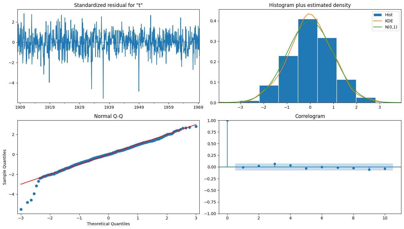
sar.plot_diagnostics(figsize=(14, 8))
plt.tight_layout();
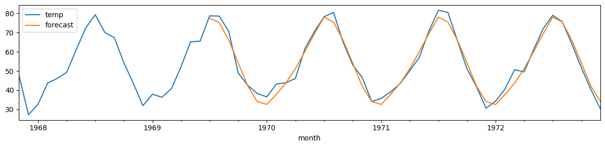
monthly_temp['forecast'] = sar.predict(start = 750, end= 792, dynamic=False)
monthly_temp[730:][['temp', 'forecast']].plot(figsize=(12, 3))
plt.tight_layout();
print(f"MSE: {mse(monthly_temp['temp'][-42:],monthly_temp['forecast'][-42:]):.2f}")
MSE: 9.23
AutoARIMA#
At this point it should be clear that identifying the optimal SARIMA model is difficult.
It requires careful analysis, trial and errors, and some experience.
The following cheatsheet summarizes some rules of thumb to select the model.
Cheatsheet for coefficients setting
ACF Shape |
Indicated Model |
|---|---|
Exponential, decaying to zero |
AR model. Use the PACF to identify the order of the AR model. |
Alternating positive and negative, decaying to zero |
AR model. Use the PACF to identify the order. |
One or more spikes, rest are essentially zero |
MA model, order identified by where plot becomes zero. |
Decay, starting after a few lags |
Mixed AR and MA (ARMA) model. |
All zero or close to zero |
Data are essentially random. |
High values at fixed intervals |
Include seasonal AR term. |
No decay to zero |
Series is not stationary. |
An alternative to manual model selection is to use automated procedures.
Here enters AutoARIMA.
AutoARIMA requires you to specify the maximum range of values to try.
Afterwards, it tries to find the best confgiuration among the possible ones.
See here for a complete list and description of the options available.
# Split the data into train and test sets
train, test = monthly_temp[:750].temp, monthly_temp[750:].temp

# Use auto_arima to find the best ARIMA model
model = pm.auto_arima(train,
                      start_p=0, start_q=0,
                      test='adf',       # Use adftest to find optimal 'd'
                      max_p=2, max_q=2, # Maximum p and q
                      m=12,             # Seasonality
                      start_P=0, start_Q=0,
                      max_P=2, max_Q=2, # Maximum p and q
                      seasonal=True,    # Seasonal ARIMA
                      d=None,           # Let model determine 'd'
                      D=1,              # Seasonal difference
                      trace=True,       # Print status on the fits
                      error_action='ignore',
                      suppress_warnings=True,
                      stepwise=True)    # Stepwise search to find the best model
Performing stepwise search to minimize aic
 ARIMA(0,0,0)(0,1,0)[12] intercept   : AIC=4558.569, Time=0.06 sec
ARIMA(1,0,0)(1,1,0)[12] intercept : AIC=4318.918, Time=0.55 sec
 ARIMA(0,0,1)(0,1,1)[12] intercept   : AIC=inf, Time=2.03 sec
 ARIMA(0,0,0)(0,1,0)[12]             : AIC=4556.588, Time=0.07 sec
 ARIMA(1,0,0)(0,1,0)[12] intercept   : AIC=4531.290, Time=0.13 sec
ARIMA(1,0,0)(2,1,0)[12] intercept : AIC=4230.055, Time=1.60 sec
ARIMA(1,0,0)(2,1,1)[12] intercept : AIC=inf, Time=3.29 sec
ARIMA(1,0,0)(1,1,1)[12] intercept : AIC=inf, Time=1.39 sec
ARIMA(0,0,0)(2,1,0)[12] intercept : AIC=4256.241, Time=1.12 sec
ARIMA(2,0,0)(2,1,0)[12] intercept : AIC=4230.500, Time=2.12 sec
ARIMA(1,0,1)(2,1,0)[12] intercept : AIC=4228.386, Time=2.28 sec
ARIMA(1,0,1)(1,1,0)[12] intercept : AIC=4317.592, Time=0.83 sec
ARIMA(1,0,1)(2,1,1)[12] intercept : AIC=inf, Time=4.82 sec
ARIMA(1,0,1)(1,1,1)[12] intercept : AIC=inf, Time=2.36 sec
ARIMA(0,0,1)(2,1,0)[12] intercept : AIC=4232.657, Time=1.32 sec
ARIMA(2,0,1)(2,1,0)[12] intercept : AIC=4230.040, Time=3.81 sec
ARIMA(1,0,2)(2,1,0)[12] intercept : AIC=4229.928, Time=2.22 sec
ARIMA(0,0,2)(2,1,0)[12] intercept : AIC=4232.612, Time=1.70 sec
ARIMA(2,0,2)(2,1,0)[12] intercept : AIC=4231.411, Time=3.98 sec
ARIMA(1,0,1)(2,1,0)[12] : AIC=4226.467, Time=0.73 sec
ARIMA(1,0,1)(1,1,0)[12] : AIC=4315.652, Time=0.35 sec
ARIMA(1,0,1)(2,1,1)[12] : AIC=inf, Time=3.74 sec
ARIMA(1,0,1)(1,1,1)[12] : AIC=inf, Time=1.37 sec
ARIMA(0,0,1)(2,1,0)[12] : AIC=4230.780, Time=0.34 sec
ARIMA(1,0,0)(2,1,0)[12] : AIC=4228.164, Time=0.38 sec
ARIMA(2,0,1)(2,1,0)[12] : AIC=4228.121, Time=1.19 sec
ARIMA(1,0,2)(2,1,0)[12] : AIC=4228.009, Time=0.52 sec
ARIMA(0,0,0)(2,1,0)[12] : AIC=4254.407, Time=0.33 sec
ARIMA(0,0,2)(2,1,0)[12] : AIC=4230.723, Time=0.51 sec
ARIMA(2,0,0)(2,1,0)[12] : AIC=4228.598, Time=0.53 sec
 ARIMA(2,0,2)(2,1,0)[12]             : AIC=4229.492, Time=1.27 sec

Best model:  ARIMA(1,0,1)(2,1,0)[12]
Total fit time: 46.954 seconds
# Summarize the model
print(model.summary())
# Forecast future values
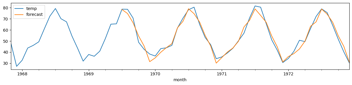
monthly_temp['forecast'] = model.predict(n_periods=len(test))
monthly_temp[730:][['temp', 'forecast']].plot(figsize=(12, 3))
plt.tight_layout();
print(f"MSE: {mse(monthly_temp['temp'][-42:],monthly_temp['forecast'][-42:]):.2f}")
                                      SARIMAX Results
===========================================================================================
Dep. Variable:                                   y   No. Observations:                  750
Model:             SARIMAX(1, 0, 1)x(2, 1, [], 12)   Log Likelihood               -2108.234
Date:                             Fri, 01 May 2026   AIC                           4226.467
Time:                                     09:23:48   BIC                           4249.487
Sample:                                 01-01-1907   HQIC                          4235.344
                                      - 06-01-1969
Covariance Type:                               opg
==============================================================================
                 coef    std err          z      P>|z|      [0.025      0.975]
------------------------------------------------------------------------------
ar.L1          0.5814      0.144      4.027      0.000       0.298       0.864
ma.L1         -0.4101      0.162     -2.528      0.011      -0.728      -0.092
ar.S.L12      -0.6818      0.029    -23.405      0.000      -0.739      -0.625
ar.S.L24      -0.3479      0.030    -11.737      0.000      -0.406      -0.290
sigma2        17.5740      0.668     26.315      0.000      16.265      18.883
===================================================================================
Ljung-Box (L1) (Q):                   0.03   Jarque-Bera (JB):               145.56
Prob(Q):                              0.87   Prob(JB):                         0.00
Heteroskedasticity (H):               0.76   Skew:                            -0.39
Prob(H) (two-sided):                  0.04   Kurtosis:                         5.03
===================================================================================

Warnings:
[1] Covariance matrix calculated using the outer product of gradients (complex-step).
MSE: 11.12
AutoARIMA or not AutoARIMA?#
While being very convenient, like all automated procedures auto_arima comes with drawbacks.
auto_arimacan be computationally expensive, especially for large datasets and when exploring a wide range of models.
Automated model selection lacks the qualitative insights a human might bring to the modeling process.
These, include understanding business cycles, external factors, or anomalies in the data.
The defaults in
auto_arimamay not be optimal for all time series data.The range of values to explore should be adjusted properly each time.
This might become almost as tricky as doing manual model selection.
auto_arimarequires a sufficiently long time series to accurately identify patterns and seasonality.
The selection of the best model is typically based on statistical criteria such as AIC or BIC.
These, might not always align with practical performance metrics such as MSE.
Grid search#
Selecting the best ARIMA model is as much an art as it is a science, involving iteration and refinement.
A common approach is to select a set of candidates for \((p,d,q)\times (P,D,Q,s)\) and fit a model for each possible combination.
For each fit model:
Analyze the residuals using the visual techniques and the statistical tests discussed before.
Evaluate the prediction performance. 🤔 How?
Evaluate its complexity. 🤔 How?
Prediction performance#
Use MSE and/or MAPE to evaluate the prediction performance of the model.
Mean Squared Error (MSE)
MSE is the average of the squared differences between the observed values and the predictions.
\(MSE = \frac{1}{n}\sum_{i=1}^{n}(Y_i - \hat{Y}_i)^2\), where \(Y_i\) is the actual observation and \(\hat{Y}_i\) is the forecasted value.
In SARIMA model selection, a model with a lower MSE is preferred, indicating better fit to the data.
Mean Absolute Percentage Error (MAPE)
MAPE is the average of the absolute percentage errors of forecasts.
\(MAPE = \frac{100\%}{n}\sum_{i=1}^{n}\left|\frac{Y_i - \hat{Y}_i}{Y_i}\right|\), where \(Y_i\) is the actual observation and \(\hat{Y}_i\) is the forecasted value.
MAPE expresses errors as a percentage, making it straightforward to understand the magnitude of forecasting errors.
If you are comparing models that predict different quantities (e.g., dollars vs. units sold), the percentage error allows for a more apples-to-apples comparison.
Also, when you’re more interested in the relative size of the errors than in their absolute size, MAPE is relevant.
Finally, MAPE is useful when the magnitude of the data varies significantly.
Model complexity#
Use AIC or BIC to estimate the model’s complexity.
Akaike Information Criterion (AIC)
AIC is a measure of the relative quality of statistical models for a given set of data.
It deals with the trade-off between the goodness of fit of the model and the complexity of the model.
\(AIC = 2k - 2\ln(\hat{L})\), where \(k\) is the number of parameters in the model, and \(\hat{L}\) is the maximized value of the likelihood function for the model.
The model with the lowest AIC value is preferred, as it fits the data well but is not overly complex.
Bayesian Information Criterion (BIC)
Similar to AIC, the BIC is another criterion for model selection, but it introduces a stronger penalty for models with more parameters.
\(BIC = \ln(n)k - 2\ln(\hat{L})\), where \(n\) is the number of observations, \(k\) is the number of parameters, and \(\hat{L}\) is the maximized likelihood.
A lower BIC value indicates a better model, preferring simpler models to complex ones, especially as the sample size \(n\) increases.
Restricting the search with Exploratory Data Analysis (EDA)#
Grid search can be very expensive if done exaustively, especially on limited hardware.
An Exploratory Data Analysis can help to significantly reduce the number of candidates to try out.
Selecting the candidates for differentiation#
Let’s start by identifying all the candidates for seasonal and general differencing.
In this case, we already know that the main seasionality is \(s=12\).
Should we apply first the general or the seasonal differencing?
If seasonal patterns are dominant and the goal is to remove seasonality before addressing any trend, start with seasonal differencing.
This is particularly useful when the seasonal pattern is strong and clear.
If the trend is the predominant feature, you might start with standard differencing.
In our case, we go with seasonal differencing first.
# create all combinations of differencing orders, applying seasonal differencing first and then general differencing
def differencing(timeseries, s, D_max=2, d_max=2):

    # Seasonal differencing from 0 to D_max
    seas_differenced = []
    for i in range(D_max+1):
        timeseries.name = f"d0_D{i}_s{s}"
        seas_differenced.append(timeseries)
        timeseries = timeseries.diff(periods=s)
    seas_df = pd.DataFrame(seas_differenced).T

    # General differencing from 0 to d_max
    general_differenced = []
    for j, ts in enumerate(seas_differenced):
        for i in range(1,d_max+1):
            ts = ts.diff()
            ts.name = f"d{i}_D{j}_s{s}"
            general_differenced.append(ts)
    gen_df = pd.DataFrame(general_differenced).T

    # concatenate seasonal and general differencing dataframes
    return pd.concat([seas_df, gen_df], axis=1)
# create the differenced series
diff_series = differencing(monthly_temp['temp'], s=12, D_max=2, d_max=2)
diff_series
| d0_D0_s12 | d0_D1_s12 | d0_D2_s12 | d1_D0_s12 | d2_D0_s12 | d1_D1_s12 | d2_D1_s12 | d1_D2_s12 | d2_D2_s12 | |
|---|---|---|---|---|---|---|---|---|---|
| month | |||||||||
| 1907-01-01 | 33.3 | NaN | NaN | NaN | NaN | NaN | NaN | NaN | NaN |
| 1907-02-01 | 46.0 | NaN | NaN | 12.7 | NaN | NaN | NaN | NaN | NaN |
| 1907-03-01 | 43.0 | NaN | NaN | -3.0 | -15.7 | NaN | NaN | NaN | NaN |
| 1907-04-01 | 55.0 | NaN | NaN | 12.0 | 15.0 | NaN | NaN | NaN | NaN |
| 1907-05-01 | 51.8 | NaN | NaN | -3.2 | -15.2 | NaN | NaN | NaN | NaN |
| ... | ... | ... | ... | ... | ... | ... | ... | ... | ... |
| 1972-08-01 | 75.6 | -4.9 | -4.9 | -3.4 | -10.3 | -2.3 | 1.7 | 1.1 | 8.4 |
| 1972-09-01 | 64.1 | -1.7 | -2.5 | -11.5 | -8.1 | 3.2 | 5.5 | 2.4 | 1.3 |
| 1972-10-01 | 51.7 | 0.6 | 2.7 | -12.4 | -0.9 | 2.3 | -0.9 | 5.2 | 2.8 |
| 1972-11-01 | 40.3 | -1.5 | 3.4 | -11.4 | 1.0 | -2.1 | -4.4 | 0.7 | -4.5 |
| 1972-12-01 | 30.3 | -0.3 | 3.2 | -10.0 | 1.4 | 1.2 | 3.3 | -0.2 | -0.9 |
792 rows × 9 columns
Filter-out non-stationary candidates#
Among all the differenced time series, keep only those that are stationary (according to ADF).
# create a summary of test results of all the series
def adf_summary(diff_series):
    summary = []

    for i in diff_series:
        # unpack the results
        a, b, c, d, e, f = adfuller(diff_series[i].dropna())
        g, h, i = e.values()
        results = [a, b, c, d, g, h, i]
        summary.append(results)

    columns = ["Test Statistic", "p-value", "#Lags Used", "No. of Obs. Used",
               "Critical Value (1%)", "Critical Value (5%)", "Critical Value (10%)"]
    index = diff_series.columns
    summary = pd.DataFrame(summary, index=index, columns=columns)

    return summary
# create the summary
summary = adf_summary(diff_series)

# filter away results that are not stationary
summary_passed = summary[summary["p-value"] < 0.05]
summary_passed
| Test Statistic | p-value | #Lags Used | No. of Obs. Used | Critical Value (1%) | Critical Value (5%) | Critical Value (10%) | |
|---|---|---|---|---|---|---|---|
| d0_D0_s12 | -6.481466 | 1.291867e-08 | 21 | 770 | -3.438871 | -2.865301 | -2.568773 |
| d0_D1_s12 | -12.658082 | 1.323220e-23 | 12 | 767 | -3.438905 | -2.865316 | -2.568781 |
| d0_D2_s12 | -10.416254 | 1.751310e-18 | 14 | 753 | -3.439064 | -2.865386 | -2.568818 |
| d1_D0_s12 | -12.302613 | 7.391771e-23 | 21 | 769 | -3.438882 | -2.865306 | -2.568775 |
| d2_D0_s12 | -15.935084 | 7.651998e-29 | 17 | 772 | -3.438849 | -2.865291 | -2.568767 |
| d1_D1_s12 | -11.846173 | 7.390517e-22 | 20 | 758 | -3.439006 | -2.865361 | -2.568804 |
| d2_D1_s12 | -18.352698 | 2.234953e-30 | 21 | 756 | -3.439029 | -2.865371 | -2.568810 |
| d1_D2_s12 | -12.221559 | 1.104309e-22 | 20 | 746 | -3.439146 | -2.865422 | -2.568837 |
| d2_D2_s12 | -15.080476 | 8.468854e-28 | 20 | 745 | -3.439158 | -2.865427 | -2.568840 |
# output indices as a list
index_list = pd.Index.tolist(summary_passed.index)

# use the list as a condition to keep stationary time-series
passed_series = diff_series[index_list].sort_index(axis=1)
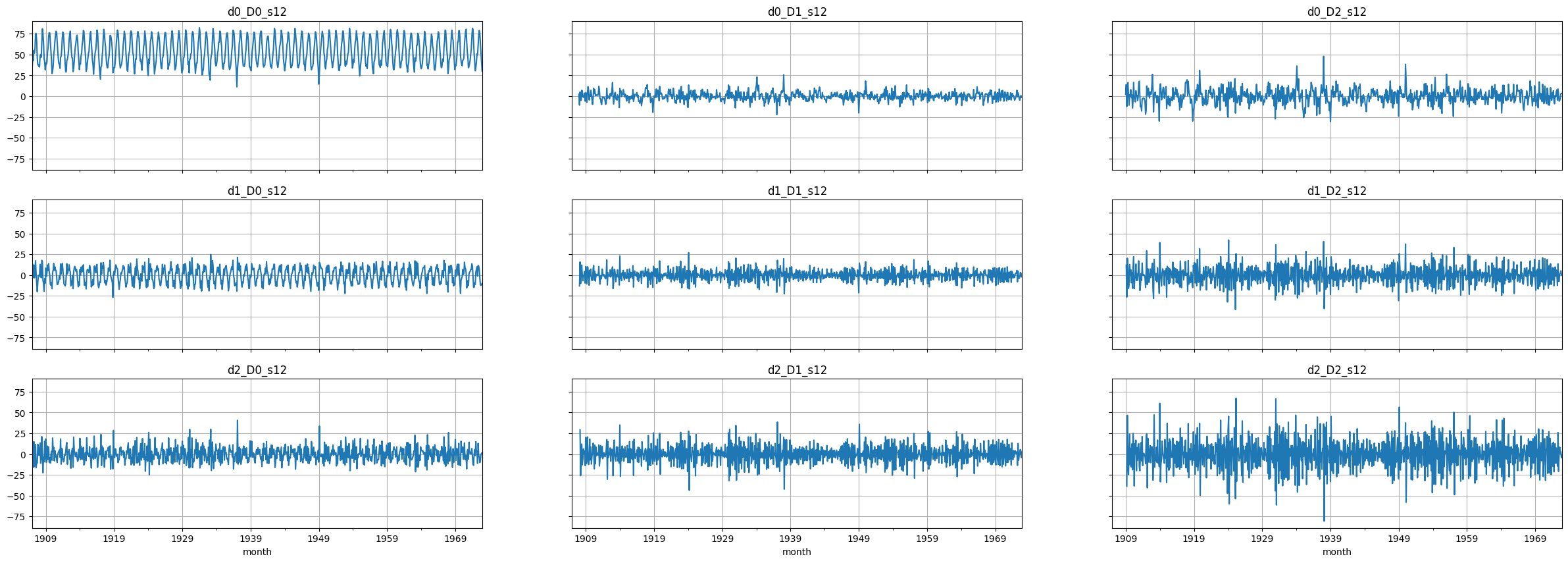
# Plot the final set of time series
# NOTE: these plots are too small. Make a larger plot for each series to see things better!
fig, axes = plt.subplots(3, 3, figsize=(30, 10), sharex=True, sharey=True)
for i, ax in enumerate(axes.flatten()):
    passed_series.iloc[:,i].plot(ax=ax)
    ax.set_title(passed_series.columns[i])
    ax.grid()
Select candidates for \(p, q, P, Q\)#
We are going to make a script to extract candidates for the orders of the AR and MA component, both in the general and the seasonal part.
We will leverage the ACF and PACF functions.
So far, we looked at the
acf_plotandpacf_plot.Now we need to use
acfandpacf.We need to understand how these relate.
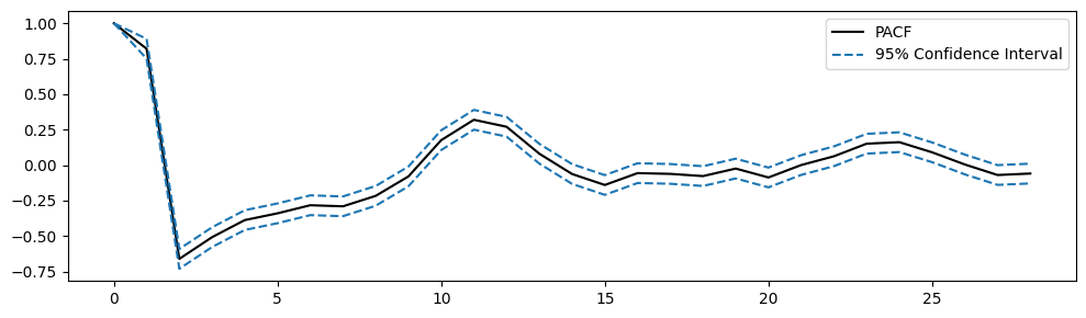
PACF, PACF_ci = pacf(passed_series.iloc[:,0].dropna(), alpha=0.05)

# Plot PACF
plt.figure(figsize=(10,3))
plt.plot(PACF, color='k', label='PACF')
plt.plot(PACF_ci, color='tab:blue', linestyle='--', label=['95% Confidence Interval', ''])
plt.legend()
plt.tight_layout();
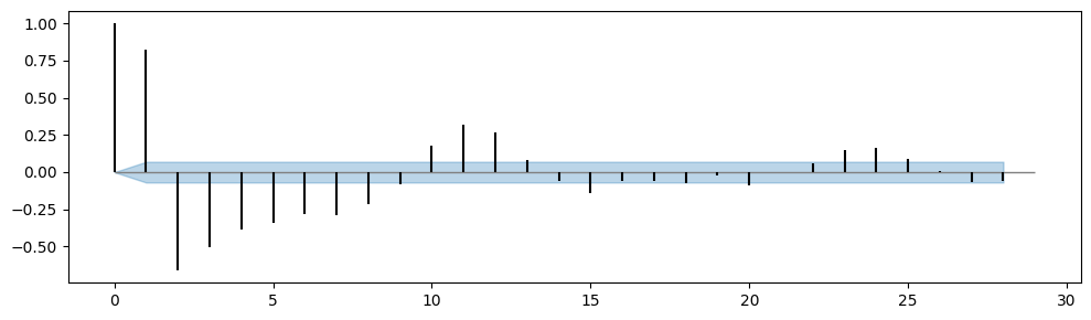
# subtract the confidence interval from the PACF to center the CI in zero
plt.figure(figsize=(10,3))
plt.fill_between(range(29), PACF_ci[:,0] - PACF, PACF_ci[:,1] - PACF, color='tab:blue', alpha=0.3)
plt.hlines(y=0.0, xmin=0, xmax=29, linewidth=1, color='gray')

# Display the PACF as bars
plt.vlines(range(29), [0], PACF[:29], color='black')
plt.tight_layout();
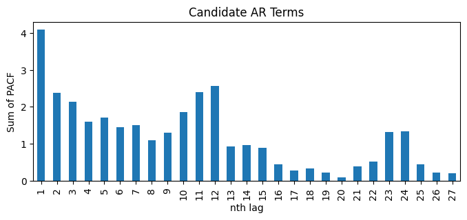
df_sp_p = pd.DataFrame() # create an empty dataframe to store values of significant spikes in PACF plots
for i in passed_series:
    # unpack the results into PACF and their CI
    PACF, PACF_ci = pacf(passed_series[i].dropna(), alpha=0.05, method='ywm')
    # subtract the upper and lower limits of CI by PACF to centre CI at zero
    PACF_ci_ll = PACF_ci[:,0] - PACF
    PACF_ci_ul = PACF_ci[:,1] - PACF
    # find positions of significant spikes representing possible value of p & P
    sp1 = np.where(PACF < PACF_ci_ll)[0]
    sp2 = np.where(PACF > PACF_ci_ul)[0]
    # PACF values of the significant spikes
    sp1_value = abs(PACF[PACF < PACF_ci_ll])
    sp2_value = PACF[PACF > PACF_ci_ul]
    # store values to dataframe
    sp1_series = pd.Series(sp1_value, index=sp1)
    sp2_series = pd.Series(sp2_value, index=sp2)
    df_sp_p = pd.concat((df_sp_p, sp1_series, sp2_series), axis=1)
df_sp_p = df_sp_p.sort_index() # Sort the dataframe by index
# visualize sums of values of significant spikes in PACF plots ordered by lag
df_sp_p.iloc[1:].T.sum().plot(kind='bar', title='Candidate AR Terms', xlabel='nth lag', ylabel='Sum of PACF', figsize=(8,3));
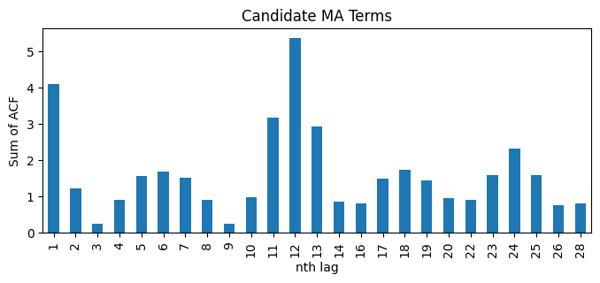
df_sp_q = pd.DataFrame()
for i in passed_series:
    # unpack the results into ACF and their CI
    ACF, ACF_ci = acf(passed_series[i].dropna(), alpha=0.05)
    # subtract the upper and lower limits of CI by ACF to centre CI at zero
    ACF_ci_ll = ACF_ci[:,0] - ACF
    ACF_ci_ul = ACF_ci[:,1] - ACF
    # find positions of significant spikes representing possible value of q & Q
    sp1 = np.where(ACF < ACF_ci_ll)[0]
    sp2 = np.where(ACF > ACF_ci_ul)[0]
    # ACF values of the significant spikes
    sp1_value = abs(ACF[ACF < ACF_ci_ll])
    sp2_value = ACF[ACF > ACF_ci_ul]
    # store values to dataframe
    sp1_series = pd.Series(sp1_value, index=sp1)
    sp2_series = pd.Series(sp2_value, index=sp2)
    df_sp_q = pd.concat((df_sp_q, sp1_series, sp2_series), axis=1)
df_sp_q = df_sp_q.sort_index() # Sort the dataframe by index
# visualize sums of values of significant spikes in ACF plots ordered by lags
df_sp_q.iloc[1:].T.sum().plot(kind='bar', title='Candidate MA Terms', xlabel='nth lag', ylabel='Sum of ACF', figsize=(8,3));
Define the grid of values to search#
# possible values
p = [1, 2, 3]
d = [0, 1]
q = [1, 2]
P = [0, 1]
D = [0, 1, 2]
Q = [0, 1]
s = [12]

# create all combinations of possible values
pdq = list(product(p, d, q))
PDQm = list(product(P, D, Q, s))

print(f"Number of total combinations: {len(pdq)*len(PDQm)}")
Number of total combinations: 144
Train the models#
We defined a function that takes every model configuration and trains a model.
For each model, we save the MSE, MAPE, AIC and BIC.
warnings.simplefilter("ignore")
def SARIMA_grid(endog, order, seasonal_order):

    # create an empty list to store values
    model_info = []

    #fit the model
    for i in tqdm(order):
        for j in seasonal_order:
            try:
                model_fit = SARIMAX(endog=endog, order=i, seasonal_order=j).fit(disp=False)
                predict = model_fit.predict()

                # calculate evaluation metrics: MAPE, RMSE, AIC & BIC
                MAPE = (abs((endog-predict)[1:])/(endog[1:])).mean()
                MSE = mse(endog[1:], predict[1:])
                AIC = model_fit.aic
                BIC = model_fit.bic

                # save order, seasonal order & evaluation metrics
                model_info.append([i, j, MAPE, MSE, AIC, BIC])
            except:
                continue

    # create a dataframe to store info of all models
    columns = ["order", "seasonal_order", "MAPE", "MSE", "AIC", "BIC"]
    model_info = pd.DataFrame(data=model_info, columns=columns)
    return model_info
# create train-test-split
train = monthly_temp['temp'].iloc[:int(len(monthly_temp)*0.9)]
test = monthly_temp['temp'].iloc[int(len(monthly_temp)*0.9):]
start = time.time()

# fit all combinations into the model
model_info = SARIMA_grid(endog=train, order=pdq, seasonal_order=PDQm)

end = time.time()
print(f'time required: {end - start :.2f}')
time required: 361.36
Analyze the results#
Show the 10 best models according to the performance (MSE, MAPE) and model complexity (AIC, BIC).
# 10 least MAPE models
least_MAPE = model_info.nsmallest(10, "MAPE")
least_MAPE
| order | seasonal_order | MAPE | MSE | AIC | BIC | |
|---|---|---|---|---|---|---|
| 141 | (3, 1, 2) | (1, 1, 1, 12) | 0.069030 | 16.777121 | 3860.336381 | 3896.733587 |
| 45 | (1, 1, 2) | (1, 1, 1, 12) | 0.069051 | 16.774448 | 3855.633789 | 3882.931693 |
| 129 | (3, 1, 1) | (1, 1, 1, 12) | 0.069079 | 16.741055 | 3856.095057 | 3887.942613 |
| 81 | (2, 1, 1) | (1, 1, 1, 12) | 0.069124 | 16.802785 | 3857.201467 | 3884.499372 |
| 135 | (3, 1, 2) | (0, 1, 1, 12) | 0.069126 | 16.792647 | 3859.554678 | 3891.402233 |
| 39 | (1, 1, 2) | (0, 1, 1, 12) | 0.069130 | 16.781200 | 3854.507890 | 3877.256144 |
| 123 | (3, 1, 1) | (0, 1, 1, 12) | 0.069167 | 16.746331 | 3854.845092 | 3882.142997 |
| 93 | (2, 1, 2) | (1, 1, 1, 12) | 0.069172 | 16.805176 | 3860.077580 | 3891.925136 |
| 75 | (2, 1, 1) | (0, 1, 1, 12) | 0.069203 | 16.811203 | 3856.176150 | 3878.924404 |
| 33 | (1, 1, 1) | (1, 1, 1, 12) | 0.069219 | 16.826980 | 3856.770561 | 3879.518815 |
# 10 least MSE models
least_MSE = model_info.nsmallest(10, "MSE")
least_MSE
| order | seasonal_order | MAPE | MSE | AIC | BIC | |
|---|---|---|---|---|---|---|
| 129 | (3, 1, 1) | (1, 1, 1, 12) | 0.069079 | 16.741055 | 3856.095057 | 3887.942613 |
| 123 | (3, 1, 1) | (0, 1, 1, 12) | 0.069167 | 16.746331 | 3854.845092 | 3882.142997 |
| 45 | (1, 1, 2) | (1, 1, 1, 12) | 0.069051 | 16.774448 | 3855.633789 | 3882.931693 |
| 141 | (3, 1, 2) | (1, 1, 1, 12) | 0.069030 | 16.777121 | 3860.336381 | 3896.733587 |
| 39 | (1, 1, 2) | (0, 1, 1, 12) | 0.069130 | 16.781200 | 3854.507890 | 3877.256144 |
| 135 | (3, 1, 2) | (0, 1, 1, 12) | 0.069126 | 16.792647 | 3859.554678 | 3891.402233 |
| 81 | (2, 1, 1) | (1, 1, 1, 12) | 0.069124 | 16.802785 | 3857.201467 | 3884.499372 |
| 93 | (2, 1, 2) | (1, 1, 1, 12) | 0.069172 | 16.805176 | 3860.077580 | 3891.925136 |
| 75 | (2, 1, 1) | (0, 1, 1, 12) | 0.069203 | 16.811203 | 3856.176150 | 3878.924404 |
| 87 | (2, 1, 2) | (0, 1, 1, 12) | 0.069289 | 16.825129 | 3859.565035 | 3886.862940 |
# 10 least AIC models
least_AIC = model_info.nsmallest(10, "AIC")
least_AIC
| order | seasonal_order | MAPE | MSE | AIC | BIC | |
|---|---|---|---|---|---|---|
| 3 | (1, 0, 1) | (0, 1, 1, 12) | 0.080283 | 61.491561 | 3846.181890 | 3864.386211 |
| 9 | (1, 0, 1) | (1, 1, 1, 12) | 0.080153 | 61.471329 | 3846.879649 | 3869.635051 |
| 15 | (1, 0, 2) | (0, 1, 1, 12) | 0.080286 | 61.482998 | 3847.914835 | 3870.670236 |
| 51 | (2, 0, 1) | (0, 1, 1, 12) | 0.080283 | 61.485309 | 3847.985625 | 3870.741026 |
| 99 | (3, 0, 1) | (0, 1, 1, 12) | 0.080295 | 61.449767 | 3848.292676 | 3875.599158 |
| 21 | (1, 0, 2) | (1, 1, 1, 12) | 0.080146 | 61.461761 | 3848.568559 | 3875.875041 |
| 57 | (2, 0, 1) | (1, 1, 1, 12) | 0.080145 | 61.464331 | 3848.650342 | 3875.956824 |
| 117 | (3, 0, 2) | (1, 1, 1, 12) | 0.080080 | 61.400462 | 3849.040154 | 3885.448796 |
| 105 | (3, 0, 1) | (1, 1, 1, 12) | 0.080096 | 61.430629 | 3849.069448 | 3880.927010 |
| 63 | (2, 0, 2) | (0, 1, 1, 12) | 0.080282 | 61.469826 | 3849.361800 | 3876.668282 |
# 10 least BIC models
least_BIC = model_info.nsmallest(10, "BIC")
least_BIC
| order | seasonal_order | MAPE | MSE | AIC | BIC | |
|---|---|---|---|---|---|---|
| 3 | (1, 0, 1) | (0, 1, 1, 12) | 0.080283 | 61.491561 | 3846.181890 | 3864.386211 |
| 9 | (1, 0, 1) | (1, 1, 1, 12) | 0.080153 | 61.471329 | 3846.879649 | 3869.635051 |
| 15 | (1, 0, 2) | (0, 1, 1, 12) | 0.080286 | 61.482998 | 3847.914835 | 3870.670236 |
| 51 | (2, 0, 1) | (0, 1, 1, 12) | 0.080283 | 61.485309 | 3847.985625 | 3870.741026 |
| 27 | (1, 1, 1) | (0, 1, 1, 12) | 0.069317 | 16.836788 | 3855.817086 | 3874.015689 |
| 99 | (3, 0, 1) | (0, 1, 1, 12) | 0.080295 | 61.449767 | 3848.292676 | 3875.599158 |
| 21 | (1, 0, 2) | (1, 1, 1, 12) | 0.080146 | 61.461761 | 3848.568559 | 3875.875041 |
| 57 | (2, 0, 1) | (1, 1, 1, 12) | 0.080145 | 61.464331 | 3848.650342 | 3875.956824 |
| 63 | (2, 0, 2) | (0, 1, 1, 12) | 0.080282 | 61.469826 | 3849.361800 | 3876.668282 |
| 39 | (1, 1, 2) | (0, 1, 1, 12) | 0.069130 | 16.781200 | 3854.507890 | 3877.256144 |
We can check if there are overlaps between the 4 different groups using the
setfunction.
set(least_MAPE.index) & set(least_MSE.index)
{39, 45, 75, 81, 93, 123, 129, 135, 141}
set(least_AIC.index) & set(least_BIC.index)
{3, 9, 15, 21, 51, 57, 63, 99}
set(least_MSE.index) & set(least_AIC.index)
set()
Show the top model according to each metric.
# the best model by each metric
L1 = model_info[model_info.MAPE == model_info.MAPE.min()]
L2 = model_info[model_info.MSE == model_info.MSE.min()]
L3 = model_info[model_info.AIC == model_info.AIC.min()]
L4 = model_info[model_info.BIC == model_info.BIC.min()]

best_models = pd.concat((L1, L2, L3, L4))
best_models
| order | seasonal_order | MAPE | MSE | AIC | BIC | |
|---|---|---|---|---|---|---|
| 141 | (3, 1, 2) | (1, 1, 1, 12) | 0.069030 | 16.777121 | 3860.336381 | 3896.733587 |
| 129 | (3, 1, 1) | (1, 1, 1, 12) | 0.069079 | 16.741055 | 3856.095057 | 3887.942613 |
| 3 | (1, 0, 1) | (0, 1, 1, 12) | 0.080283 | 61.491561 | 3846.181890 | 3864.386211 |
| 3 | (1, 0, 1) | (0, 1, 1, 12) | 0.080283 | 61.491561 | 3846.181890 | 3864.386211 |
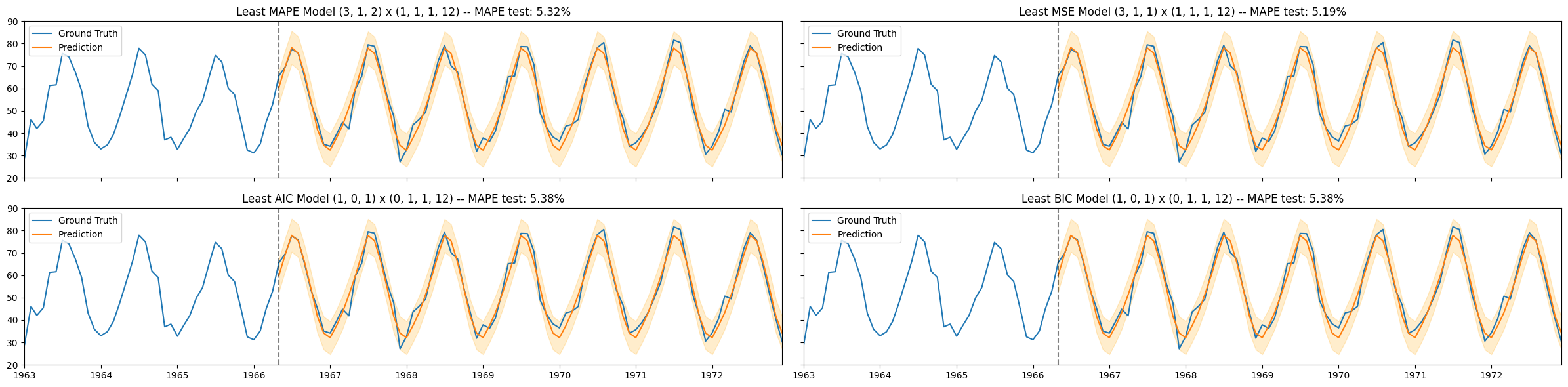
Compute performance on the test set#
Take the best models, compute the predictions and evaluate their performance in terms of MAPE on the w.r.t. test data.
# Take the configurations of the best models
ord_list = [tuple(best_models.iloc[i,0]) for i in range(best_models.shape[0])]
s_ord_list = [tuple(best_models.iloc[i,1]) for i in range(best_models.shape[0])]
preds, ci_low, ci_up, MAPE_test = [], [], [], []

# Fit the models and compute the forecasts
for i in range(4):
    model_fit = SARIMAX(endog=train, order=ord_list[i],
                        seasonal_order=s_ord_list[i]).fit(disp=False) # Fit the model
    pred_summary = model_fit.get_prediction(test.index[0],
                                            test.index[-1]).summary_frame() # Compute preds
    # Store results
    preds.append(pred_summary['mean'])
    ci_low.append(pred_summary['mean_ci_lower'][test.index])
    ci_up.append(pred_summary['mean_ci_upper'][test.index])
    MAPE_test.append((abs((test-pred_summary['mean'])/(test)).mean()))
# visualize the results of the fitted models
fig, axs = plt.subplots(nrows=2, ncols=2, figsize=(24,6), sharex=True, sharey=True)
titles = [f'Least MAPE Model {ord_list[0]} x {s_ord_list[0]}',
          f'Least MSE Model {ord_list[1]} x {s_ord_list[1]}',
          f'Least AIC Model {ord_list[2]} x {s_ord_list[2]}',
          f'Least BIC Model {ord_list[3]} x {s_ord_list[3]}']
k = 0
for i in range(2):
    for j in range(2):
        axs[i,j].plot(monthly_temp['temp'], label='Ground Truth')
        axs[i,j].plot(preds[k], label='Prediction')
        axs[i,j].set_title(titles[k] + f' -- MAPE test: {MAPE_test[k]:.2%}')
        axs[i,j].legend()
        axs[i,j].axvline(test.index[0], color='black', alpha=0.5, linestyle='--')
        axs[i,j].fill_between(x=test.index, y1=ci_low[k], y2=ci_up[k], color='orange', alpha=0.2)
        axs[i,j].set_ylim(bottom=20, top=90)
        axs[i,j].set_xlim(left=monthly_temp.index[-120], right=monthly_temp.index[-1])
        k += 1
plt.tight_layout()
plt.show()
Summary#
Autoregressive Moving Average (ARMA) models.
Autoregressive Integrated Moving Average (ARIMA) models.
SARIMA models (ARIMA model for data with seasonality).
Selecting the best model.
Exercise#
Look at sensor data that tracks atmospheric CO2 from continuous air samples at Mauna Loa Observatory in Hawaii. This data includes CO2 samples from March 1965 to December 1980.
co2 = pd.read_csv('https://zenodo.org/records/10951538/files/arima_co2.csv?download=1',
                  header = 0,
                  names = ['idx', 'co2'],
                  skipfooter = 2)

# convert the column idx into a datetime object and set it as the index
co2['idx'] = pd.to_datetime(co2['idx'])
co2.set_index('idx', inplace=True)

# Rmove the name "idx" from the index column
co2.index.name = None
co2
| co2 | |
|---|---|
| 1965-01-01 | 319.32 |
| 1965-02-01 | 320.36 |
| 1965-03-01 | 320.82 |
| 1965-04-01 | 322.06 |
| 1965-05-01 | 322.17 |
| ... | ... |
| 1980-08-01 | 337.19 |
| 1980-09-01 | 335.49 |
| 1980-10-01 | 336.63 |
| 1980-11-01 | 337.74 |
| 1980-12-01 | 338.36 |
192 rows × 1 columns
Determine the presence of main trend and seasonality in the data.
Determine if the data are stationary.
Split the data in train (90%) and test (10%).
Find a set of SARIMAX candidate models by looking at the ACF and PACF.
Perform a grid search on the model candidates.
Select the best models, based on performance metrics, model complexity, and normality of the residuals.
Compare the best model you found with the one from autoarima.